Reference no: EM133119088

MAE 3319 Dynamic Systems Modeling and Simulation - The University of Texas at Arlington

Assignment

This course pertains to modeling and analysis of engineering systems which means deriving and solving differential and algebraic equations that are used to determine the performance of the engineering system. A controls course follows this modeling course. The controls course pertains to stabilizing or improving the performance of the engineering system by adding feedback to the model.

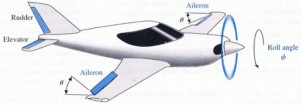
A schematic of an airplane with a feedback roll control system is shown below. Feedback is achieved with a gyro that measures angular rotation rate and instrumentation that measures aileron angles. The roll control computer in the airplane receives a desired roll angle Φ_d from the pilot and then the computer moves the ailerons θ to achieve the desired roll angle in a reasonable time with minimal oscillations.

An controls engineer has modeled the aerodynamics and then designed the feedback controller gains to achieve these objectives. The model also includes the aerodynamic effects associated with turbulence T(t) that cause the roll angle to undesirably change during flight. Thus, there are two possible inputs that affect the roll angle of the airplane: (1) desired roll angle Φ_d(t) from the pilot and (2) turbulence T(t). The equations for the roll dynamics and the feedback controller are

Φ¨ + Φ^· = T + θ Roll dynamics due to turbulence and ailerons
θ^· = u Aileron change rate based on feedback control u
u = 64(Φ_d - Φ) - 35Φ^· - 7θ Feedback control u

For the following parts to this assignment, create a function file and keep adding to it each part as you work through the assignment. In the end, you will have a single function file that does every part of the assignment.

Question 1: Define state variables for the equations and express the three equations in state variable format assuming that Φ(t) is the output-of-interest. Let x₁ = Φ, x₂ = Φ^· and x₃ = θ

x^· = Ax + B and y = Cx + D A = ? B = ? C = ? D = ?

Question 2: Enter this system into MATLAB using the command ‘ss' and use ‘damp' to determine the eigenvalues. Define the system with notation R.

Confirm that the eigenvalues are -2.18 and -2.91 ± j4.57 using damp(R)?

What is the damping ratio?

What are the time constants?

Question 3: Use the command ss2tf(A,B,C,D,1) to get the transfer function for input T and ss2tf(A,B,C,D,2) to get the transfer function for input Φ_d. Confirm that both transfer functions have the same denominator and thus, the same eigenvalues.

Question 4: What is the DC gain of the Φ_d transfer function?

What does this mean in terms of what the roll angle will be eventually if the input from the pilot is a constant?

Question 5: If the pilot puts in a step input for Φd, assuming T = 0, how long will it take for the roll angle to reach steady state?

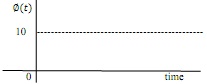
Question 6: Assume Φ_d(t) is a step of 10 degrees and T=0. Assume the initial roll angle is zero. Considering the damping ratio, the damped natural frequency, the final value and the time constants, draw an estimate of the airplane roll angle following the command Φ_d(t) = 10.

Question 7: Use MATLAB to generate the roll angle response to a pilot command of 10 degrees and determine if it matches your estimated plot in part 6. If it doesn't match, determine which one is wrong.

Question 8: To see what happens if the airplane flies through a very small tornado, assume T(t) is a unit impulse. Use the impulse command for T(t) assuming Φ_d(t) = 0 and all initial conditions are zero to generate a plot of Φ(t).

Does the feedback controller bring the disturbed roll angle Φ(t) back to zero and in a timely manner?

Question 9: Turbulence, T(t), is a stochastic process containing many frequencies. A typical plot of T(t) is shown below. It is very random and contains many frequencies.

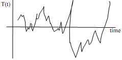
If you don't understand the meaning of ‘containing many frequencies', review Fourier series on page 26 in Section 1.9. So, T(t) can be represented by the sum of sine and cosine terms at many frequencies. The question is, which of these frequencies have a significant affect on the roll angle?

A very important concept pertaining to frequency response is bandwidth. For example, the bandwidth for a set of audio speakers is the input frequency range that the output is not distorted; in this case you have a desired input and desired output that you don't want distorted and the larger the bandwidth, the better.

However, for problems such as this roll control system, the turbulence input is not desired and the resulting disturbance to the roll angle is not desired. Thus, it is desired that the transfer function for the input T(t) has a low bandwidth which means that as many frequencies as possible of the turbulence will be ignored or at least have a reduced effect on the roll angle.

The industry standard for the definition of bandwidth is the frequency range for which the dynamic gain is not less than 3 dB below the zero-frequency dynamic gain. Thus, according to this definition, all contributions of the input with frequencies not in the bandwidth of the transfer function will theoretically not affect the roll angle.

Use ‘bode' in MATAB to show that the bandwidth of the T transfer function is approximately 2.89 rad/s. That is, according to the industry standard of -3 dB, all turbulence input frequencies greater than 2.89 rad/s can be ignored.

Question 10: To demonstrate the significance on the amplitude of the output for frequencies below, at, and above the bandwidth, assume Φ_d(t) = 0 and use ‘lsim' in MATLAB to generate Φ(t) for T(t) = 640/7sin(0.3t), for T(t) = 640/7sin(3t) and for T(t) = 640/7sin(30t); put all three responses on the same plot for comparison. Note, to see a significant portion of the steady-state response, your simulations need to run more than 5-time constants; Use a final time of 12 s. In addition, the highest input frequency is 3 rad/s; so, to get at least 20 points per cycle with this frequency, the time increment for all three simulations needs to be about 0.01 s.

(10.a) From the frequency response plot, we see that a turbulence input frequency of 0.3 rad/s has a dynamic gain that is very close to the DC gain of the transfer function; from your lsim simulation, what is the steady-state roll angle amplitude for this low frequency?

(10.b) If the frequency of the turbulence input is equal to the bandwidth frequency, 3 rad/s, from your lsim plot what is the steady-state roll angle amplitude?
Is this amplitude consistent with the -3 dB gain reduction associated with the bandwidth frequency?

(10.c) Considering your lsim plot for a turbulence frequency of 30 rad/s, what is the roll angle amplitude?

What can you say about the ability of the roll angle control system to filter out (ignore) turbulence with frequencies above the bandwidth?
Considering the comparison of the amplitudes of the three plots, what can you conclude about the significance of the bandwidth?

Question 11: In this part of the assignment, the turbulence input is a band limited white noise (Sections 8.3.4.2, 8.3.5.4 and example on page 285) with magnitude of 50 for 0 < f < 10 hz i.e.

Upload the function file StochInput in the March 28 Announcement. Copy and paste it as an internal function in the function file you are creating for this assignment. In the dpsd function at the end of StochInput, change the desired PSD to the one shown above.

(11.a) Determine appropriate values for N and H (Section 8.3.5.1).

(11.b) Generate a stochastic input for the turbulence that has this PSD. StochInput should generate plots of the turbulence and the desired PSD so you can confirm you entered the correct PSD.

(11.c) Run lsim with this input to the turbulence transfer function. Plot the roll angle Φ(t) resulting from the airplane flying through this turbulence.

(11.d) Use the MATLAB function files ‘mean' and ‘std' to compute the mean and standard deviation of Φ(t).