Machine and power systems laboratory assignment

Assignment Help MATLAB Programming

Reference no: EM133369512

Introduction to Electrical Machine and Power Systems Laboratory Assignment

Pre-Lab

The laboratory experiments for this course are simulation-based using MATLAB software. MATLAB is licensed. Students can access and use MATLAB if the lab session will be conducted in a computer lab. For home practices, students are recommended to use the MATLAB equivalent, Octave. In both situation of using MATLAB or Octave, the MATLAB sample programs may be required editing to run to produce the desired results.

If the lab session will be conducted on face-to-face basis in the computer lab, MATLAB will be used as the simulation software. Students are required to strictly follow the SOP set by the university. Besides, students are encouraged to bring own storage media to save the developed scripts for home practices.

If the lab session will be conducted online in Microsoft Teams (MT), the MATLAB equivalent, Octave will be used. Students are required to perform the following before the session.
1. To confirm the lab session in respective course in MT.
2. To install Octave in individual Windows computer. The software can be obtained.
3. In the case of unsuccess installation, students can access the cloud-based Octave but it is not encouraged as limitations may be incurred during the lab session and help documents are not available.
4. Upon the success installation, To start Octave with GUI, students can run "Octave-5.2.0 (GUI)".
5. Students can refer to menu HELP Documentations On disk. The Octave manual is available and students should familiarize the software by going thorough first two topics, A Brief Introduction to Octave and Getting Started.

The recommended handbook is essential which is the following title:

Jimmie J. Cathey, (2001). Electric Machines: Analysis and Design Applying MATLAB. McGraw-Hill. The book's website, www.mhhe.com/engcs/electrical/cathey, includes all the MATLAB programs in the text for download.

Title: Power factor correction

Objective: To perform the power factor correction and identify the required capacitance.

Software: Octave or Octave Online

Procedure:

1. run "Octave-5.2.0 (GUI)".

2. As an example of the practice, Example 2.19 from the recommended handbook is performed using Octave. Students may use the programs as in Appendix to begin the simulation of the example.

3. Let us calculate current flows through a branch with the impedance Z_L=3+j4 as shown in the following figure. The voltage we apply is V=240+j0.

2072_Power Systems Laboratory.jpg

* The figure numbering follows from source of reference, i.e. the recommended textbook.

4. The program we run is cquot3.m. You are required to copy the codes in Appendix. Then press "New script" in the menu and paste to the new script. Save the new script with the file name of "cquot3.m".

5. Run the program by pressing the Run button. Student is required to enter some data on the command window and the following results will be displayed on the command window:
>> cquot3

PROGRAM DIVIDES COMPLEX NUMBERS
Form: 1-polar, 2-rectangular How many numbers to be divided? 2 Form of 1 = 2
Real 1 = 240
Imag 1 = 0

Form of 2 = 2
Real 2 = 3
Imag 2 = 4

QUOTIENT = 28.8 +j -38.4 = 48|_-53.1301deg I_Re = 28.8
I_Im = -38.4
I_Mag = 48
I_Arg = -0.9273
>>

6. The results could be interpreted as: The current comprises of a real part with magnitude 28.8 A, and an imaginary part of -38.4 A. The current magnitude of 48 A

is lagging the applied voltage, 240?0° V, by an angle of -53.1301°. The cosine of this angle is the power factor.

7. Next, we calculate the apparent power, real power and reactive power using the following program. This program calculates the powers and the required capacitance based on the targeted power factor. Note that complex power is the product of two complex numbers, i.e. voltage and the conjugate of current.

8. Repeat steps 4 and 5 and the results on the command window as shown in the following:
>> cpower3

PROGRAM MULTIPLIES TWO COMPLEX NUMBERS

Complex number 1
Form: 1-polar, 2-rectangular Type of input voltage '1 or 2'? = 1
Mag 1 = 240
Deg 1 = 0

Complex number 2
Form: 1-polar, 2-rectangular Type of input Current '1 or 2'? = 1
Mag 1 = 48
Deg 1 = -53.13

PRODUCT = 6912.0165 +j 9215.9877 = 11520|_53.13deg
P_watt = 6912.0165
Q_var = 9215.9877
S_VA = 11520
S_rad = 53.13
How much is targeted power factor? 0.9 phi = 0.45103
Q_new = 3347.6424
Q_C = 5868.3453
omega = 376.99
omegaVV = 21714688.42161
CVV = 0.00027025
>>

9. The results could be interpreted as: The complex power is given by
S= P+ jQ=6912.0165+ j 9215.9877=11520 ∠ 53.13 °.

Adding a power factor correction capacitance in parallel, if can target a power factor of 0.9, and the VARs supplied by the source becomes

Q'/P = tan (cos^-1 (0.9))=tan (25.84°)

Q' = P tan( cos^-1(0.9))=3347.6424 VARs

The reactive power that must be supplied by the capacitor is

Q_C = Q-Q' = 9215.9877 - 3347.6424 = 5868.3453

The source angular frequency is given by ω = 2Πf =2Π 60, and the capacitance C required is equal to

C = Q_C/ωV²= 5868.3453/2Π60(240)² = 270.25 μF

10. The results can be verified by:

At 60 Hz, the susceptance due to the power factor correction capacitance is

B_C = 2Π60 × (207.25 × 10^-6) = 0.101882 S

The current flow is easily calculated:

~I_C = V_s ~ Y_C = (240 ? 0 ° ) (0.101882 ∠ 90 ° ) A.

11. We run the program cprod.m to determine the current flow through the power factor correction capacitance which is attached in parallel with the RL network. The results are as follow.

>> cprod

PROGRAM MULTIPLIES COMPLEX NUMBERS

Form: 1-polar, 2-rectangular
How many numbers to be multiplied? 2 Form of 1 = 2
Real 1 = 240
Imag 1 = 0

Form of 2 = 1
warning: Matlab-style short-circuit operation performed for operator & warning: called from
cprod3 at line 14 column 4
Mag 2 = 0.10188185
Deg 2 = 90

PRODUCT = 1.4972e-15 +j 24.4516 = 24.4516|_90deg
P_watt = 1.4972e-15 Q_var = 24.4516
S_VA = 24.4516
S_rad = 90
>>

12. Next, the sum of current flow through the RL network and the power factor correction capacitance is calculated. They are extracted from the above results.

~I = ~I_RL +~I_C = 28.8- j 38.4 + j 24.4516=28.8- j 13.9484=32 ∠ (-25.8417) A

The power factor after correction is given by cos(-25.8417°)=0.9. This result verifies the outcome of the simulation.

13. The computation above is an example of a single-phase power factor correction. You must present the results as a three-phase power factor correction. The Unit Practice Laboratory Exercise requirement is as follow.

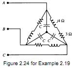
14. Power Factor Correction Practice Simulation Exercise:
Capacitors C are added to the 50-Hz, three-phase network of Figure 2.24 to correct the input power factor to the following conditions. You are required to determine the value of C and find the total kVAR rating of the capacitor bank if V AB=480 V. Check the results by performing the full analysis. (You may modify the codes to demonstrate and visualize the desired results).
i. Unity
ii. 0.95 lagging
iii. 0.9 leading

15. Write a short report to discuss your answers. Your report should contain a short introduction, some explanations on the effect of different power factors, your experimental procedure, and the results you obtain at every stages of the simulation. The rubric is provided to assist your report writing.

Reference no: EM133369512

Questions Cloud

Describe the perception of scale : Describe the perception of scale you read from it, how that scale is conveyed, and how the use of shape, composition, line type,

What greatly impacts the re-election of a sitting president : What greatly impacts the re-election of a sitting president? Name three desires most people have for government finances. How do liberal and conservative

Personal definition of good art : Carefully consider your own, personal definition of "good" art. Then, locate a work of art that you believe constitutes "good" visual art

Make a list of 5 things the president said someone : Make a list of 5 things the President said someone might think were positive or good for the nation and people. Explain why some might think this for each

Machine and power systems laboratory assignment : Introduction to Electrical Machine and Power Systems Laboratory Assignment - determine the current flow through the power factor correction capacitance

Unique characteristics of ancient greek figurative sculpture : Discuss the unique characteristics of ancient Greek figurative sculpture as it developed from the Archaic period through the Classical period

Explain the statement, correlation is not a cause : Explain the statement, "correlation is not a cause".

What do you think will be the most common element across : What do you think will be the most common element across the staff members of a congressional office? Think about workplace or someplace you would like

What you see as their benefits to participate : Consider one of the issues of the day that is currently being considered by Congress. Identify one interest group supporting or opposing that issue.

User Account

All Pages