Reference no: EM133141696

FE 621 Computational Methods in Finance - Stevens Institute of Technology

Problem 1. Finite difference approximations.

Recall that forward and centered finite-difference approximations for the derivative of a function f are given by

Δ_h⁽¹⁾f(x) = (f (x + h) - f (x))/h , Δ_h⁽⁰⁾f (x) = f (x + h) - 2f (x) + f (x - h)/2h.

(a) Other useful finite-difference approximations can be constructed in similar ways. Show that

Δ_hf (x) = 1/6h (2f (x + h) + 3f (x) - 6f (x - h) + f (x - 2h)),

approximates f'(x) up to an error term of order O(h³).

(b) Define the finite-difference approximation errors:
e_h⁽¹⁾(x) = f'(x) - Δ_h⁽¹⁾f (x),
e_h⁽⁰⁾(x) = f'(x) - Δ_h⁽⁰⁾f (x),
e_h(x) = f'(x) - Δ_hf (x).

For the function f (x) = sin(x) and x₀ = 1, plot the above errors as a function of h on a log-log scale. That is, plot log |e_h⁽¹⁾(x₀)|, log |e_h⁽⁰⁾(x0)| and log |e_h(x0)| as a function of log h.

(c) What are the slopes in your three graphs? Are they in line with what we should expect from theoretical results?

Problem 2. Explicit methods.

In the Black-Scholes model, the price v(t, s) of a European option with payoff Φ satisfies the Black-Scholes PDE:

v_t(t, s) + rsvs(t, s) + σ²s²/2.v_ss(t, s) - rv(t, s) = 0,

v(T, s) = Φ(s).

The solution can be shown to be of the form v(t, s) = ertu(t, ln s), where u(t, x) satisfies:

u_t(t, x) + (r - σ²/2)u_x(t, x) + σ²/2.u_xx (t, x) = 0,

u(T, x) = e^-rT Φ(e^x).

It is typically better to solve the above constant-coefficient PDE rather than the standard Black-Scholes PDE.
• Use the explicit method to solve the constant coefficient PDE for a put option.
• Use parameters K = 10, r = 0.05, σ = 0.20 and T = 0.5.
• Report your option price approximations for:
(i) Initial stock price S0 ranging from S = 4 to S¯ = 16.
(ii) α < 0.5, α = 0.5 and α > 0.5, where α = σ²δt/2δx² .
You can report your results graphically and/or using a table (see, for example, Table 1 in the course notes).
• Compare your results to exact prices computed using the Black-Scholes formula. Comment on your findings. Explain how you would extend your algorithm to price an American put option and identify the optimal exercise boundary. Explain briefly the meaning of the exercise boundary for American options.

Problem 3. Implicit methods.

Consider the same setup as in Problem 2. In this problem we use the fully implicit method to compute the prices of American put options.

(a) Use a forward difference for time-derivatives and a centered difference for space-derivatives to show that the finite-difference equation at node (tm, xn) can be written as

(α + β)u˜^m_n+1 + (1 - 2β)u˜_n^m + (-α + β)u˜_n-1^m = u_n˜^m+1,

where

α = -(r - σ²/2)δt/2δx,      β = - σ²/2. δt/(δx)²

(b) The equation above for n = N - 1 and n = -N + 1 involves the boundary values u_N^m and u_-N^m. Reasonable boundary conditions for a put option are v_s(t, s) = 0 as s → ∞ and v (t, s) → -1 for s →0. for u(t, x) these conditions translate to

u_N^m = u_-N^m                  u_-N^m = u_-N+1^m + (δx)e^-rtm e^X-N.

Use this to rewrite the finite-difference equations for n = N 1 and n = N + 1 and show that all the equations can be written in matrix form as

Cu^~m = b^m+1

where C is a tridiagonal matrix,

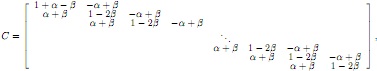
and bm+1 is a column vector given by

(c) Optional (extra credit): Argue that for small δt and δx, the matrix C is diagonally dominant. It is known that such matrices are invertible, which ensures that the system Cu˜^m = b^m+1 has a unique solution. Hint: Use that for small δt and δx, β is much larger than α in absolute value.

(d) Solve the system of equations using Thomas' algorithm (LU-decomposition) and report your option price results in the same way as in Problem 1, using the same parameter values. Consider values of α larger than 0.5 and see whether the prices remain accurate.