Reference no: EM132243944

PROJECT - CONSTRUCTING AN OPTIMAL PORTFOLIO

The main objective of this project is to learn how to construct an optimal portfolio of risky securities. In course of the project you need to choose the optimal amount to invest in each of these assets (i.e. choose portfolio weights) using mean variance optimization framework - the cornerstone of modern portfolio theory.

Project Plan and Deliverables -

I. Data Description

You will work with returns on 12 risky assets. Table 1 outlines the data sources and requirements:

Table 1: Data

Type of Assets	Data Source
Returns on two hedge fund indices	Select two hedge fund indices. The data are compiled by Credit Suisse. You can download these data from the Credit Suisse website:
Returns on ten other risky assets such as stocks, stock indices, ETFs, etc.	Your assets must cover different industries and, perhaps, even countries. You can use WRDS database, specifically CRSP. This database contains financial returns on all publicly traded companies (but there is a time lag). If you want to work with more recent data use Bloomberg or any other professional website (note: Yahoo Finance is not one of them). Name the source (or sources) of your data.

1. Describe how the two strategies behind your two selected hedge fund indices work.

2. Explain reasons that prompted you to select these two strategies.

3. Provide a brief description of other portfolio assets (stocks, ETFs, etc.) and justify their inclusion in your portfolio:

a. You can present a comprehensive analysis of the status and outlook of the global economy and explain it relates to your assets.

b. You can also focus on characteristics of individual assets.

II. Past performance

The main goal of this part of the project is to use data on past returns to estimate mean returns, and the variance-covariance matrix of assets in your portfolio.

Download data on monthly returns for the most recent 5-year period on your assets from the CRSP or other databases into the Excel file. Make sure that your dates are consistent across all assets, i.e. you select returns for the same 5-year period.

1. Using commands in the Excel Functions menu (click on fx button), calculate expected monthly returns on all stocks (use AVERAGE function).

2. Calculate the variance - covariance matrix.

You can calculate the variance-covariance matrix using cov-matrix.xlam application, posted on BB. You need to download this application onto your computer and then open it within your Excel program. Don't forget to enable macros. You will see capital letter M appearing in the right corner of the Excel menu bar when you click on the Data tab:

If you have N assets in your portfolio, the Variance-Covariance is an N by N table. On the diagonal of this matrix are variances, on off-diagonal are covariances, each covariance appears twice since Cov(x,y) = Cov (y,x).

The steps are:

a. Decide on the location of the matrix in the Excel spreadsheet and highlight N by N area. If you want to include labels in the first row (for example ticker symbols for your stocks or names of the hedge fund indexes) then highlight (N+1) by (N+1) area since your first row and your first column will be taken by labels.

b. Click on the covariance matrix icon in the menu bar. The following window will open:

c. Enter your Input range (your monthly returns)

d. Select "Labels in First Row" if you want them.

e. Enter output range (your N by N or (N+1) by (N+1) area).

f. Click OK

3. Annualize expected returns, standard deviations, variances and covariances. It means you have to multiply monthly expected returns, variances and covariances by 12. We can do this because we assume markets to be efficient at least in a weak form. Market efficiency means that monthly returns are independent of each other; that is the correlation coefficient between returns in one month and returns in any other month is 0. Annualized standard deviation is a square root of the annualized variance.

You can multiply the entire variance-covariance matrix by 12.

4. In your Briefing Book report monthly and annual expected returns and standard deviations. Present the annualized variances- covariance matrix.

5. Calculate and present the correlation matrix.

i. On the Data tab, click Data Analysis.

If you can't find the Data Analysis button, you need to load the Analysis ToolPak add-in.

ii. Select Correlation and click OK.

iii. In the Correlation window enter the data range, check on Labels if you want them, select the output range, and click OK.

6. Discuss these statistics you reported in Part II.

III. Optimal Portfolio Selection

The main objective of this part of the project is to learn to use mean-variance optimization framework to construct the efficient frontier. The efficient frontier is the set of the optimal portfolios. Each portfolio on the frontier is optimal in a sense that it provides the highest possible expected return per unit of risk. You need to use the Solver optimization package in Excel to complete this part. You can also use any other programming language and write your own optimization program. In this case, please attach you code in the appendix of the Briefing Book

Assume that you have $10 million to invest in risky assets.

In Excel, the steps are

Step 1: Open the Excel spreadsheet which contains annualized expected returns on your assets and the annualized variance-covariance matrix.

Below, in N columns specify weights of the N assets in your portfolio. You can start with any set of numbers for weights. They will change after you run Solver.

the next (N+1)^th column, enter a sum of weights formula (use =SUM( ) command in Excel). We will use this cell to set up a constraint: _i=1∑^Nw_i = 1

This constraint simply states that weights of any portfolio should sum to 1.

Step 2: In the next three columns enter the formulas for the variance, standard deviation and expected return (in that order) of a portfolio:

Since you are dealing with fairly large portfolios, the more efficient way to calculate variance of a portfolio and its expected return is to use matrices and matrix multiplication commands in Excel.

We will use the following matrix form for equation (1):

σ_p² = ωΩω' (4)

In equation (4), ω denotes 1 by N row vector of weights, Ω stands for N by N variance-covariance matrix, and ω' is a transpose of ω, i.e. a N by 1 column vector of weights.

To do this in Excel:

(i) Use the following command in Excel to perform matrix multiplication to find the variance of your first portfolio.

=MMULT(MMULT(1 by N range of cells for the weight vector ω, N by N range of cells for var-covar matrix Ω),TRANSPOSE(1 by N range of cells for the weight vector ω))

Press simultaneously CTRL-SHIFT and while holding these two keys, also press ENTER.

(ii) In the next cell calculate the standard deviation of your portfolio, which is just a square root of the variance.

(iii) In the cell next to the one with the standard deviation, calculate the expected return on your portfolio. In the matrix notation, equation (2) becomes:

E[R^~_p] = Eω' (5)

In (5) E stands for the 1 by N row vector of expected returns and ω' is a column N by 1 vector of weights (i.e. transpose of the row vector ω).

To do this in Excel, write:

=MMULT(1 by N range of cells for the vector of the expected returns E, TRANSPOSE(1 by N range of cells for the vector of weights ω))

Do not forget to press simultaneously CTRL-SHIFT and while holding these two keys, also press ENTER.

When you write the Excel version of the variance formula (4) and expected return formula (5), "lock" the addresses of cells, which contain the variance-covariance matrix and the vector of expected returns. Do not lock addresses of cells which contain weights.

(iv) Copy everything 10 times (next ten rows). Notice that addresses of the cells where you have weights change, but the cells for variance-covariance matrix and the vector of expected returns are locked and remain the same.

Step 3: Use Solver to find the weights of the minimum variance efficient (MVE) portfolio of your chosen stocks in the first row. This is a portfolio with the lowest possible variance constructed using your N assets.

To do this, you simply minimize the variance of the portfolio, no constraints on the expected return of the portfolio needed.

a. Go to Data, find Analysis and click on Solver.

b. In Solver window, in "Set Objective", enter the address of the cell where you have your variance function for the first portfolio and click on Min. Your objective is to minimize the variance of the portfolio.

c. In "By Changing Cells" enter the range of weights that Solver can change. Make sure that you do not restrict short sales, i.e. don't check the box for positive values. Negative weights simply mean that you have a short position.

d. Add the constraint on weights: In the reference cell place, enter the address of the cell where you have the sum of weights formula and set it to equal to 1.

e. Click OK. The weight constraint appears in the constraint window.

f. Now click on Solve.

Step 4: Use Solver to calculate efficient portfolios for each level of expected returns. That is, increase expected returns above the level of E[RMVE] in small increments (for example, the next portfolio's expected return would be 1% higher than the expected return on the MVE portfolio). This new return enters Solver as your constraint. You need to find a portfolio that has the smallest possible variance (and standard deviation) and pays your chosen expected return. Mathematically, you solve the following optimization problem:

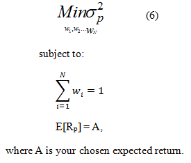
You will need to repeat your optimization with Solver 10 more times, each time increasing the expected return by 1%. Don't use paste and copy at this point.

In Solver, the steps are exactly the same as in Step 3, except that in the "Subject to constraints" window, you now need to add the return constraint.

a. Click on "Add". The constraint window will open.

b. In the "Cell Reference", enter the address of the cell which contains the expected return on the next portfolio after MVE pf. and choose =.

c. In the "Constraint" enter = address of cell containing the expected return on the MVE pf and add 1% to it: E[r_MVE]+0.01. This means that return on your next portfolio should be equal to the return on MVE portfolio plus 1%.

d. Click on "OK."

Deliverables for Part III -

1. In your briefing book, in your own words, describe the optimization problem that you solve with the help of Solver (or any other program) to determine the weights of assets in the Minimum Variance Efficient (MVE) portfolio:

a. What function are you minimizing?

b. What variables are you choosing?

c. Are there any constraints?

2. Report the weight of each risky asset in the MVE portfolio, the expected return and standard deviation of this portfolio.

3. Describe the problem, which you solve to find the weights of assets in other 10 efficient portfolios. Report weights of your other ten efficient portfolios, their expected returns and standard deviations. (It is convenient to arrange this information into a table).

4. Now suppose that short sales are not allowed. Find the MVE portfolio with the short sale constraints in place. How does the optimization problem need to change to accommodate short sale constraints?

5. Derive the rest of the efficient frontier with short sale constraints.

6. Present the graph of efficient frontiers without short sale constraints and with short sale constraints in place. Both frontiers must be on the same graph to facilitate the comparison between them. Mark the MVE portfolio on each graph.

7. Explain how short sales constraints affect your investment opportunities. You can comment on the changes in the characteristics of the MVE portfolio and then discuss the rest of the efficient frontier.

8. Eliminate short sale constraints once again, i.e. short sales are allowed. But now construct the efficient frontier without you two hedge fund indices. Show both frontiers with and without hedge funds on the same graph to facilitate comparison between them. Comment on the contribution of your two hedge fund indices to your investment opportunities. Do they help you to increase return and diversify risk?

Attachment:- Assignment File.rar