Reference no: EM133197204
Assignment:
1. A fabric mill in rural South Carolina is the only employer in town. The figure below depicts three curves: the mill's value of marginal product of labor VMPL, labor supply, and marginal labor cost MLC. The MLC curve is drawn assuming that workers aren't unionized.
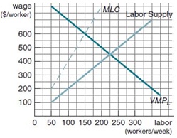
(a) If workers don't bargain collectively, the profit-maximizing mill employs _____ workers per week and pays a weekly wage of $ _____ per worker. Mark this point with an A in the figure above.
(b) The mill workers unionize and successfully bargain for a $350 wage. How does this union wage affect the mill's marginal-labor-cost curve? Carefully illustrate the two parts of the new MLC curve.
(c) How many workers are employed in the equilibrium with wu = 350? Illustrate the equilibrium with a B in the figure.
(d) A ruling by the NLRB limits the mill's ability to operate during a strike, which increases the union's bargaining strength. The union threatens to strike if the mill doesn't raise the weekly wage to $400. The mill concedes. Illustrate the new union equilibrium with a C. How does employment of union workers vary with the union wage in this model?
(e) Apply this model to predict the effect of a minimum wage in a monopsony labor market. Assume the minimum wage is less than the wage in the competitive equilibrium.
2. Here are the weekly wages in a sample of 10 wage and salary workers: 150, 250, 300, 350, 400, 450, 550, 650, 800, and 1,000.
In small samples like this one, the gaps between the wages are a source of ambiguity in computing wages at percentiles of the distribution. Let's resolve the ambiguity by using midpoints. With an even number of observations, the median is halfway between the highest value in the bottom half of the sample and the lowest value in the top half of the sample. Also, 30 percent of the workers earn $300 or less, but 30 percent also earn $349.99 or less. To be consistent with the calculation of the median wage, the wage at the 30th percentile is halfway between $300 and $350.
(a) Compute the mean and median of wages in this sample.
(b) What are the wages at the 10th and 90th percentiles in this sample?
(c) What is the 90-10 percentile ratio? That is, the worker at the 90th percentile earns _____ times as much as the worker at the 10th percentile.
(d) How far from the median wage are the wages at the 10th and 90th percentiles? Do wages in this small sample skew to the right?
3. The marginal product of effort of Mac, a typical worker in a fast-food burger joint, is one-fourth burgers per hour; that is, MPe = .25. The price of a burger is $2. The figure below graphs Mac's marginal cost of effort.
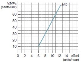
(a) If Mac increases his effort by one unit per hour, the change in the burger joint's revenue is $ ____ per hour. That is, what is VMPe, the value of Mac's marginal product of effort? Plot the VMPe curve in the figure.
(b) Mac's efficient effort ê is the solution to what equation? Illustrate the solution in the figure. Mac's efficient effort is ê = _____units of effort per hour.
(c) If the price of a burger rises from $2.00 to $2.80, what happens to Mac's efficient level of effort?
(d) If the marginal-cost-of-effort curve shifts down, what happens to ê?
(e) Suppose the market for fast-food workers like Mac is competitive. If Mac's quantity supplied of effort is efficient, how much does he earn per hour?
4. The figure below displays a market for teenage labor with a minimum wage of $6 per hour.
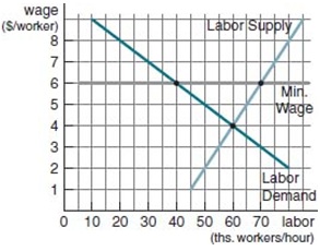
(a) How many workers are unemployed at the $6 minimum wage?
(b) The government places an hourly tax of $1 per worker on employers. Show the effect of the tax on the demand for labor.
(c) With both the minimum wage and the labor tax, how many workers do firms employ? What is the incremental effect of the tax on employment?
(d) With both the minimum wage and the labor tax, how many workers are unemployed? What is the incremental effect of the tax on unemployment?