Reference no: EM131199127
COMPUTER PROJECT
One report per group of two students. You can also choose to work alone.
The group should list their names and percentage effort on the project with both members of the group signing the sheet for verification. This sheet should be submitted with the project.
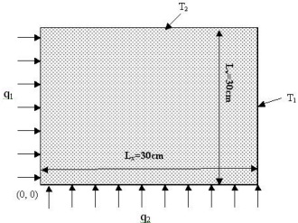
A square block (30 x 30 cm) of thickness 2 cm is held at constant temperature along two boundaries and has two heaters attached along two other boundaries which supply uniform flux to these boundaries as shown. Each heater is supplying 500W (Note the heat flux will be 500W/Area- where Area= thickness x length- 500 W/(0.02m x.3m)= 83,333 W/m2. You can choose an initial temperature for the block and the boundary conditions T1 and T2. You may also pick the material of the block and then look up its thermal properties such as k, ρ and Cp.

The Computer Project Report should be uploaded on Sakai and should include:
(1) Justification for performing two-dimensional analysis for a three dimensional object.
(2) Your finite difference equations
(a) for the four boundaries, (b) at corners if applicable, and (c) for the interior nodes.
(3) Restriction on time step for stability due to the boundary conditions using energy balance.
(4) One way to verify that your numerical solution is correct is to refine your mesh and see if your solution converges. Hence first use the number of nodes in X and Y direction to be M=N=31 and then re-run your program for M and N =61. In both cases plot the graphical temperature distribution after 360 seconds and 2000 seconds when q. = 0 and for q. = 1 W/cm3, respectively ( q. is the volumetric rate of heat generation in the block). Comment on your results.
Note that when you decrease your dx and dy, you must check your time step accordingly to meet the stability requirement.
(5) The mesh refinement will only tell you if your solution has converged but how can you ensure that it is converging to the correct physical solution? One way to verify this is to conduct a global energy balance. Do this on your steady state solution for q. = 0 and for q. = 1 W/cm3.
The approach to this is to use the final temperature distribution you obtain from your numerical solution for steady state and conduct energy balance with the entire block as your control volume by calculating the energy coming in from the boundaries (You already know the q'' for two boundaries as that is the boundary condition. For the other two boundaries where the temperature is fixed, the energy balance on the boundary cells can provide the local boundary heat flux leaving the block). The sum of all has to be equal to the energy produced within the block under steady state conditions. List the error for each case ( q. = 0 and q. = 1 W/cm3) for both meshes (M=N=31 and M=N=61).
(6) Graph the steady state temperature distribution and the minimum time it takes to reach the steady state for q. = 0 . This time is when the temperatures from one time step to the next are essentially the same at every node in your mesh.
(7) Another way to validate the numerical solution is to compare the numerical solution with the analytical solution (see, e.g., page 7 of Lecture 11 notes). Compare the steady-state numerical solution of the temperature distribution on the diagonal line from the lower-left corner to the upper right corner, to the analytical solution provided in Lecture 11 for q. = 0 .
(8) Demonstration of the numerical instability (and the concept of garbage in- garbage out) by purposely choosing a large time step and printing out the temperature distribution at t=80 seconds for q. = 0.