Reference no: EM133107844

GEEN 1125 Finite Element Applications - University of Greenwich

Principles of FEM: Virtual Domain, Meshes, Element formulation and Boundary Conditions

Learning Outcome 1: Explore the different principles that make up an FE Solution

Learning Outcome 2: Understand concept of virtual domains and how to create them.

Learning Outcome 3: Explore the role of mesh types on the solution of an FE problem.

Learning Outcome 4: Apply Element Formulation mathematics to design new elements for FE problem.

Learning Outcome 5: Understand the effect of boundary conditions on FE solutions with particular focus on periodic boundary conditions

Learning Outcome 6: Explore role of material choice in understanding the behaviour of an FE domain.

Question 1:

A fracture test specimen is shown in Figure CW2-1. The specimen is made of 4340 steel material with a Young's Modulus, E_s = 210 GPa, and Poisson ratio, v = 0.33. It has dimensions of 40 x 40 x 5 mm³. A crack is introduced on the left edge about the centreline with dimensions as shown in Figure Q6B.

The steel plate is pulled apart using the lower and the upper holes through to a Dirichlet y-axis deformation of |u_y| = 10mm. The steel plate is to be modelled using a Johnson-cook nonlinear plasticity model with model parameters given in Table CW2-1. In all cases, it is advisable to mesh finely the region around the crack tip.

A. Using an appropriate virtual domain creating software (e.g. ABAQUS, SolidWorks) of your choice, create the 3D virtual domain of the fracture test specimen.

B. Undertake the test simulation for the following three mesh discretization cases, and show contour plots from your simulation:
a. Case A: Hexahedral elements
b. Case B: Tetrahedral element
c. Case C: Wedge elements
For all three cases, show the contour plots in deformed configuration showing: von Mises stress, plastic strain and displacement magnitude.

C. Based on the three mesh discretizations above, plot on the same bar chart of the principal and average stresses in the region at the crack tip. Comment on the influence of element choice on the results obtained.

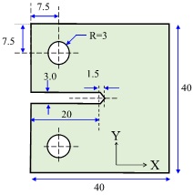
Figure CW2-1: Fracture test specimen

Question 2:

The meshed model of a bath is shown in Figure CW2-2. The bath is made of steel of Young's Modulus, E = 210 GPa. The mesh is based on 2D quadrilateral element. We are interested in developing the element formulation for our bespoke four-node quadrilateral element whose isoparametric natural coordinates are given in Figure CW2-2.

For the quadrilateral element:

A. Show derivations of the relevant element shape functions, Ni where i = 1, 2, 3, 4, needed to describe the element formulation for the quadrilateral element.

B. The plot of the four shape functions

C. Derive the resulting strain-displacement matrix, B of this element type.

D. Using the B-matrix above and material properties, derive the applicable stiffness matrix, K that will be used within the finite element solver for this new element type.

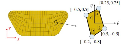
Figure CW2-2: A bath discretized with quadrilateral element. Insert shows the isoparametric natural coordinates of the bespoke quadrilateral element.

Question 3

An M-shaped specimen, shown in Figure CW2-3A, is used to determine the dynamic tensile behaviour of a steel specimen within a Split Hopkinson Pressure Bar apparatus. The dimensions of the test specimen are given in Figure CW2-3A and the specimen is made from steel with properties given in Table CW2-3A.

The upper end of the specimen is imposed with a compressive displacement, U = 3 mm while both bases are fixed securely in all X, Y and Z-axes. The side faces are fixed in XZ-plane allowing for movement only in the Y-axis. The steel plate is to be modelled using an elastoplastic material model with isotropic softening given in Table CW2-3A and damage evolution law with properties given in Table CW2-3B.

A. Create the virtual domain of the M-shaped tensile test specimen in an appropriate software of your choice. Create a nodal set for the gauge sections of the test specimen.

B. Undertake the compressive test simulation for the specimen using hexahedral elements with ELEMENT DELETION switched to ON. Show contour plots from your simulation for the Von Mises stress (MISES), equivalent plastic strain (PEEQ), displacement, (U MAGNITUDE) and actively yielding flag (AC YIELD).

C. Using simulation outputs, determine the plot of volume averaged y-stress (S22) versus y-axis strain stress (E22) for only the gauge section elements.

D. From your simulations, calculate the error between numerical and analytical yield stresses determined from your study? Discuss three sources of the errors from your study.

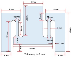
Figure CW2-3A: M-shaped test specimen dimensions

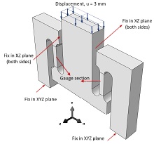
Figure CW2-3B: Isometric view of the M-shaped test specimen

Attachment:- Finite Element Applications.rar