Reference no: EM133126972

IE 505 Production Planning and Scheduling

Homework Assignment

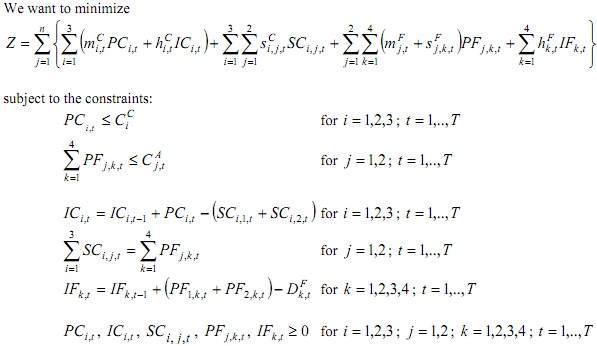
Question 1: Consider a situation in which a single finished product is produced by two assembly plants, and immediately distributed to four regional warehouses, where it is stored. All customer demand is shipped from theses regional warehouses. The system also contains three other supplying plants, which each produce the same major component part of the finished product produced at the assembly plants. Each of these component-producing plants maintains its own inventory of completed parts, which are shipped on demand to the assembly plants. The five plants and three finished product warehouses are each at a different geographical location. Production costs vary among plants and shipping costs are, of course, a function of the source and the destination. Each plant has a known capacity in each period. The problem is to specify the least-cost production and distribution plan for the system that satisfies given demand schedules for each finished product warehouse. Let
i = index for component-producing plants ( i = 1,2,3 )
j = index for assembly plant plants ( j = 1,2 )
k = index for warehouses ( k = 1,2,3,4 )
T = number of periods in the planning horizon
t = index for periods in the planning horizon ( t = 1,..,T )

C_i^C = capacity (in units) of the component-producing plant i

C_j,t^A = capacity (in units) of the assembly plant j in period t

D^F_{k ,t} = demand for finished product at warehouse k in period t

m_i,t^C = manufacturing cost to produce one unit of component part at the component producing plant i in period t

m_i,t^F = manufacturing cost to produce one unit of finished product at the assembly plant j in period t

Si_,j,t^C = shipment cost of one unit of component part from the component-producing plant i to assembly plant j in period t

S^F_{j,k ,t} = shipment cost of one unit of finished product from the assembly plant j to warehouse k in period t

h^C_i,t = inventory holding cost for one unit of component part at component-producing plant i in period

h^F_{k ,t} = inventory holding cost for one unit of finished product at warehouse k in period t

We define the following decision variables:

PC_i,t = number of units of component part produced at component-producing plant i in period t

IC_i,t = component part inventory at the component-producing plant i at the end of period t

SC_{i, j,t} = number of units of component part shipped from component-producing plant i to assembly plant j in period t

PFj,k ,t = number of units of finished product produced at assembly plant j and shipped to warehouse k in period t

IF_{k ,t} = finished product inventory at warehouse k at the end of period t

Suppose we want to modify the above model to include the following features:

- Production capacity at component-producing plants can be varied from period to period at a cost. But, in each period the capacity increase is allowed at one component-producing plant only. Let c⁺_i,t and c^-_i,t be unit costs of capacity increases and decreases, respectively, in period t . However, capacity increase or decrease in period cannot exceed 20 percent of the capacity of the previous period.

• Up to MB^F_kt units of the finished product demand at warehouse k can be backlogged at unit cost at the end of period t. Backlogging is allowed in every period except the last.

• Up to MS^C_t units of component part produced by all component-producing plants can be sold at a unit selling price of sp_t^C in period t, and up to MP_t^C units of component part can be purchased at a unit cost of pp_t^C in period t. The purchased component part is consumed in the same period it is bought. That is, it is not kept inventory for future use.

• Production lead-time is 1 period at assembly plants. That is, a unit produced in a period can be used in the next period, at the earliest.

Define the additional decision variables needed, and modify the given LP model by taking into account the features above and obtain a new model. Explain the objective function and constraints of the new model clearly.

Question 2. Consider an extension of the lot sizing problem in which there are M production sources (e.g., production plants) for satisfying the demand of a single product in each of T time periods. One unit of the product can be produced at a cost v_i,t dollars by production source i (i = 1, 2,..., M ) in period t (t = 1, 2,...,T ). When production source i is used in period t, then a fixed cost Ai,t , which is independent from the number of units produced by this source, incurs. The initial inventory level of the product is zero, and the product may be stored from period t to period t = 1 at a cost h_t dollars per unit. No shortages are allowed. D_t is the demand (in units) for the product in period t. Production source i has a capacity Cap_i,t (in units of product) in period t. The maximum number of units of product that can be stored in the warehouse of the company in any month is MS.

(a) Formulate the problem as a mixed-integer linear programming (MILP) model. Define the decision variables explicitly. Write the mathematical expressions for the objective function and constraints, and explain them clearly.

(b) To eliminate all inventory decision variables from the model in part (a), obtain an expression, which is a function of production and demand quantities only, for the inventory level at the end of each period t .

(c) Substitute the expression obtained in part (b) into the model in part (a) and modify the model in part (a) to obtain a new formulation in which all inventory decision variables are eliminated from the model in part (a). That is, write the mathematical expressions for the objective function and constraints of the modified model.

Question 3. Consider the following one-dimensional cutting stock problem where the length of the master roll is 4200 mm.

(a) Formulate a mathematical model to minimize the total number of standard sheets used for satisfying the orders.
(b) Solve the model in part (a) by GAMS. Make a tableau for illustrating the cutting plan obtained from the solution.
(c) Generate all feasible cutting patterns and calculate their wastes (in cm).
(d) Using the FFD (First Fit Decreasing) heuristic solve the problem above. Make a tableau for illustrating the cutting plan obtained from the solution.

Question 4. Consider the two-dimensional case of the cutting stock problem. A sample cutting pattern for a problem with three rectangular pieces to be cut from the standard sheet appears in the figure below. W and L are the width and length of the standard sheet, and wi and li are the width and length of the rectangular piece i to bet cut from the standard sheet. Note that there is no waste in this sample cutting pattern.

If the cuts are always continued to the end of the standard sheet, then this type of cutting is called "guillotine cut", as illustrated in the following figure for a cutting pattern of a different problem.

The minimum number of cuts in the cutting pattern above is 4. If one can determine all possible cutting patterns for a two-dimensional cutting stock problem, and use them in the mathematical model developed for the one-dimensional cutting stock problem, then two-dimensional cutting stock problem with rectangular pieces can also be solved.

Now, consider the following two-dimensional cutting stock problem where the guillotine-type cutting method is applied, and the width and length of the standard sheet are 50 cm. and 100 cm., respectively.

(a) Generate all feasible cutting patterns, illustrate them by figures, and calculate the minimum number of guillotine-type cuts for each cutting pattern.
(b) Using all feasible cutting patterns generated in part (a), formulate a mathematical model to minimize the total number of guillotine-type cuts, not the total number of standard sheets used.
(c) Solve the model in part (b) by GAMS. Make a tableau for illustrating the cutting plan obtained from the solution.