Reference no: EM13498408

A circuit with input voltage v_i(t), and output voltage v_o(t), is shown below. Also of interest is the voltage v_L2,

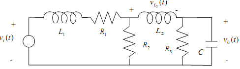
Part 1. The circuit elements have parameter values L₁ = 0.1 H, L₂ = 0.2 H,

C = (2 + 3 x 0.xyz) x10^-8 F, and R_I =1,000 ohms, R₂ =1,000 ohms, and R₃ = 10,000 ohms, where xyz are the final three digits of your student ID number. The value of 0.xyz satisfies 0≤0.xyz≤1 so the C capacitance value then lies in the range [20, 50] nF.

1. Using Kirchhoff's voltage and currents laws, derive the 3^rd order differential equation for v_o(t). Assume that there is no energy stored in the capacitor or inductors at time t = 0 . From the differential equation, find a state variable representation, and specify the state variable matrices A, B, C, D, to generate the voltages v_o(t) and v_b (t). (Note: Complete Tasks 3 and 4 to verify that your differential equation is correct.)

2. Careful study of the circuit reveals that the "dc gain" of the circuit is G_dc = (R₂ || R₃)1(R₁ + R₂ || R₃) . Use Matlab to determine the response of the circuit ( v_o(t)) over a suitable time interval (roughly [0, 0.002] sec) to input v₁(t= (1 / G_dc)u(t), where u(t) is the unit-step signal. Accurately plot the response, v_o(t), and determine (from the numerical response) the 100% rise time, percent overshoot, and 2% settling time. (Note that the default rise time value that some Matlab functions provide is the 10% to 90% rise time, so make sure your numerical result matches your plot.) Also, accurately plot v_l2(t). Verify that v_o(t) and v_L2(t) approach the correct steady-state values as t -> ∞.

3. From the differential equation, determine the transfer function H(s) - ^Vo^(s)/ V_i(s) and find v_i(s) all finite poles and zeros. Plot their location in the s-plane. Also accurately plot the transfer function frequency response (use Bode plots). Verify that the steady-state output level of the unit step-response matches the "dc gain" of the frequency response.

4. Assuming all-zero initial conditions in the circuit, use loop or node analysis in the s-domain to derive equations for the two loop currents, I₁(s) and I₂(s) . From these equations, determine the transfer function, H(s) - V_o(s)/v_i(s) , and verify that it matches V_i(s) your result in task 3.

Part 2. Set R_I = 0, R₃ -> ∞ (that is, resistors R_I and R₃ drop out of the circuit), and let the value of R₂ be R₂ = 1000 + 3000 x 0 .xyz , where xyz are the final three digits of your student ID number. R₂ is then in the range [1000, 4000] ohms.

5. Design the filter to be a 3^th-order Butterworth filter with -3 dB cutoff frequency 4.0 kHz (8,000k radians/sec). This will involve, for your specified value of R₂, properly selecting the values of L_I , L₂, and C. Note that the desired Butterworth filter transfer function must have the form H(s)  = ω_c² / S³ + 2ω_cS² + 2ω_c²S + ω³_c where ω_c is the cutoff frequency. After designing the filter, complete the following.

a. Find the pole locations (e.g., using MATLAB), and plot the pole locations in the s-plane. Identify the angle of the complex poles in the s-plane and relate the complex pole positions to the damping factor and natural frequency of the second-order factor in the denominator of the transfer function.

b. Use state variables and MATLAB to determine the unit step response. Accurately plot the step response and determine the 100% rise time, maximum percent overshoot, and 2% settling time.

c. Accurately plot the filter frequency response (Bode plots). Verify that the filter response matches the desired Butterworth filter frequency response.

d. Without computer assistance (that is, by hand calculation), determine the equation for the impulse response, h(t), the output voltage in response to an impulse input, v_i (t) = 5(t).

e. Without computer assistance, determine the equation for the unit-step response. Verify that your equation for unit-step response matches the MATLAB state variable solution in task 5b).

f. The steady-state sinusoidal response of the filter is determined by the frequency response, evaluated at the sinusoid frequency. Let the circuit input be v,.(t). sin(21r40000 u(t). Use Matlab to compute the filter response for a suitably long duration so that the response reaches (approximately) the steady-state signal. Plot in a single figure both v_; (t)and v_o(t), and identify in your figure that the expected filter magnitude and phase are realized. One way to show this would be to plot the theoretical sinusoidal steady state solution (also in the same figure) and show that v_o(t) approaches this as time gets sufficiently large. Approximately how long does it take for the (Matlab) response to reach steady-state? Compare this (observed) time to the settling time found in part 5b).

6. It is possible to design a 3^rd-order Butterworth high-pass filter by modifying your existing design (and circuit) as follows. In the circuit, replace every inductor with a capacitor, and replace every capacitor with an inductor. The high-pass filter transfer function is then related to the low-pass filter transfer function by replacing every occurrence of impedance "Ls" with the impedance "l/sC", and every occurrence of the inverse of impedance term "sC" with "I/Ls". In your derivation of the low-pass filter transfer function in task 4, with R₁ = 0 and R₃ -) CO, you should have found a low-pass transfer function of the form H_lowpass(s)= R₂/s³L₁L₂C + • • • + R₂ Making the substitutions sL_i,. ->1/sC,. and sC -> 1/sL , (and leaving R₂ unchanged) the high-pass filter has a transfer function of the form H_highpass(s) = R₂/1/s³L₁L₂C + • • • + R₂  Simplifying yields the highpass filter transfer function. In addition to this modification of the lowpass filter transfer function, use loop analysis in the s-domain (similar to task 4) to directly derive loop currents and the overall transfer function for the highpass filter, H_highpass(s) = V_o (s) / V_i (s) This can serve as an independent verification that your transfer function is correct. The resulting filter transfer function is then of the form H_highpass(s) = s³/ S³ + 2ω_cS² + 2ω_c²S + ω³c where ω_c is the highpass filter cutoff (-3 dB) frequency.

a. Select the values of C₁, C₂, and L so that your 3r^d-order Butterworth highpass filter has cutoff (-3 dB) frequency 2 kHz. Use the same value of R₂ as for the lowpass Butterworth filter. Use Matlab to generate the Bode frequency response plots for your filter. Verify that your filter has the correct cutoff frequency.

b. Use Matlab to generate the response to the input v_i(t)= cos(2Π1000t u(t).

Compare this response to the sinusoidal steady-state response, and relate the observed magnitude and phase (at steady state) to the filter frequency response.

In your report, present the results of the above tasks along with the discussion mentioned on the first page, and supporting derivations, analysis, design equations, plots, and MATLAB code. As a rule-of-thumb, the report should be sufficiently detailed so that if you were to refer to it in one year, you could easily follow the derivations, discussion, and results. Since the report must be typeset, select a suitable word processing system for your work. The LaTeX system is available for free download and is excellent, but requires some learning.