Reference no: EM131220818

Assignment 1 -

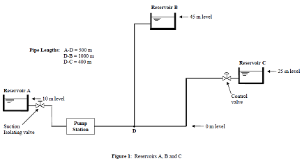
Question 1: Design a pumping system that will transfer raw water from Reservoir A to Reservoirs B and C. A control valve shall be located in Line D-C next to Reservoir C to control the share of flow between Reservoir B and C. See Figure 1.

The pump station shall contain a main suction isolation valve and at least three pumps. It shall be located some 200 m downstream of Reservoir A. The pumps shall be arranged and valves be provided and duty/standby pumps be selected as per "good design practice".

System operating modes:

MODE (I) (Design condition)

- Normal flow rate from reservoir A to be 250 litres/second

- Discharge into Reservoir B to be 50 litres/s and into Reservoir C to be 200 litres/s.

MODE (II) (All flow to Reservoir C)

- The same number of pumps running as in MODE (I)

- Control valve in Line D-C set to cause all flow running into Reservoir C, i.e. no water to be discharged into or drained from Reservoir B.

Tasks:

1. Draw a detailed system schematic for MODE (I), allowing for sufficient valves (no non-return valves in Line D-B) and at least three 90 degree bends per pipe section.

2. Show the selected pipeline diameters and their associated head losses (based on good engineering practice) in a table and justify the reasons for your component selection.

3. Show the expected pump operating points for MODE (I) and demonstrate these by showing pump performance and system resistance curves.

4. Determine the amount of the main suction isolation valve to be throttled in MODE (I) in order to match an NPSH safety factor of 1.15 for the pumps.

5. Show pump operating points, system resistance curves and control valve settings for operation in MODE (II).

QUESTION 2: From the information given below, calculate the total life cycle cost for each pipeline diameter and determine the optimum pipeline diameter.

Pipeline system parameters:

System flow rate, Q = 1000 1/s

Pipeline static lift, H_s = 500 m

Pipeline length, L_p = 80 km

Pipe friction factor, f = 0.02

System design life 30 years, NPV factor = 7.50

Cost of pumping power = $0.05/kWh

Hours of operation = 24 hours/day, 365 days/year

Pump set efficiency = 85%

Pipeline maintenance cost = $20,000 pa

Cost per pump station = $ 5,000,000

Number of pump stations = 2

Pipe diameter and costs

Pipe internal diameter Pipe supply and install cost

700 mm $600/m

800 mm $650/m

900 mm $700/m

1000 mm $750/m

In the calculation, you may wish to ignore losses in valves, fittings, inlet and outlet.

QUESTION 3: Write a factsheet or a short essay/report of literature review on the current research and development in pumping technology. You may choose to focus on one of the following topics (other topics should be pre-approved by the course examiner):

• Strategies for energy efficiency of pumping systems
• Application and importance of pumping systems

You may need to cover:

• Introduction - importance of the issue
• Technology currently being investigated (the working principle, pros and cons)
• Future research
• Summary

You may base your essay on the materials assigned for this module and also any other information available on the internet and in the library. Concise and clear to the point presentation style are strongly encouraged. The report should be well structured with appropriate uses of headings (as suggested above) and sub-headings. The key points should be clearly emphasized and the extensive uses of bullet points (dot points) or tables are encouraged.

Marks will be allocated according to the following three criteria:

• General presentation and layout, grammar, spelling, referencing, logic of the presentation.
• Accuracy/appropriateness of factual materials.
• Discussion/interpretation of materials.

Length: A standard essay format of 2-4 A4 pages (including 3-5 references) would be appropriate.

Assignment 2 - Time Response and Controller Design

Please provide your solutions to the below questions. Show all work and present your work logically, justifying all assumptions. The questions marked with an asterisk (*) include a MATLAB component.

Exercise 1: Reduction of subsystems

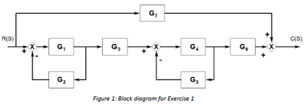
Find the transfer function T (s) = C(S)/C(R) of the block diagram in Figure given that:

G₁ = 2/(s+2), G₂ = 1/s, G₃ = 5

G₄ = ((s+5)/(s+3)(s+10)), G₅ = 2, G₆ = s, G₇ = 5/s

Also, write a MATLAB script using feedback, series and parallel commands and confirm that your handwritten answer and MATLAB agree.

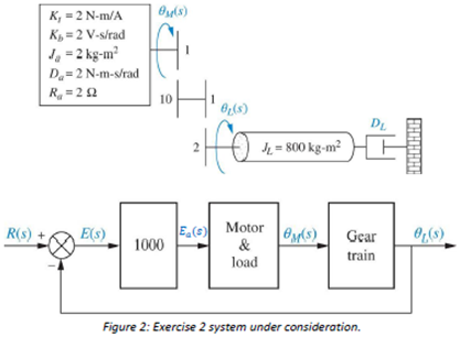
Exercise 2: What's the damping?

Consider the motor/load feedback control system shown in Figure 2 below. The load damping D_L is unknown, but when R(s) is a step, the response of θ_L has an overshoot of 20%. Do the following:

a) Find the transfer function θ_L(s)/R(s) (you'll have a D_L in your equation since you don't know it yet)

b) Calculate the damping ratio that corresponds to 20% overshoot

c) Find D_L using the information from a and b).

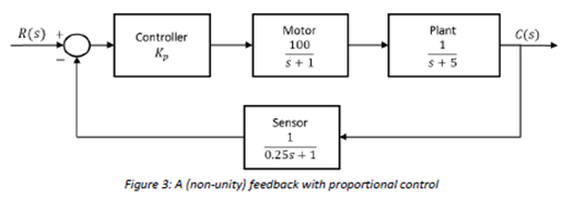
Exercise 3: A proportional controller

For the velocity control system in Figure 3:

a) Find the closed-loop transfer function T(s) = c(s)/R(s).

b) Find a value of K_p that will yield less than 10% overshoot for the closed-loop system. (Note: ignore the zero dynamics to calculate K_p initially).

c) Is the second order component of the closed-loop system dominant?

d) What is the magnitude of step input that will give a steady-state velocity of c(∞) = 50 m/s?

e) Using your K_p from part b), write a MATLAB script that calculates the closed-loop transfer function, T(s) = c(s)/R(s).

f) Simulate the step response of T(s). Is the overshoot 10% as you designed? Discuss.

Exercise 4: Linearization of a vehicle moving through air

Consider the simple model of a vehicle moving through air

mv^· = F - kv²

where v is the velocity of the vehicle, F is the forward traction force, and k is a drag parameter that depends on the properties of the air and the geometry of the vehicle. The parameters are m = 1000kg and k = 10N·s²/m². Do the following:

a) Linearize the model about the steady-state F^- = 1000N.

b) Find the transfer function v'(s)/F'(s) for the linearized system in a)

c) Consider a vehicle that is at the steady-state you found in a). A step change in the traction force is introduced, F'(s) = 200/s. Use your transfer function model to predict time response of the velocity v(t).

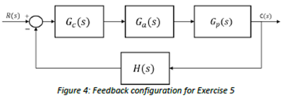
Exercise 5: Stability

Consider a unity feedback (H(s) = 1) configuration Figure 4. For the following systems, determine the range of K that will maintain stability.

(a) G_c(s) = K, G_a(s) = 1/s(s²+1), and G_p(s) = 1/(s²+s+1)

(b) G_c(s) = Ks, G_a(s) = 1/(s+1), and G_p(s) =  1/((s+2)(s+5))

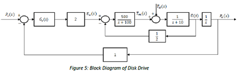
Exercise 6: Disc drive problem

Recall the disc drive problem introduced in tutorial. Last time we developed the transfer functions seen in Figure 5. Do the following:

a) Find the transfer function G_d(s) = P_o(s)/T_d(s) when G_c(s) = K_c.

b) For G_c(s) = K_p, find the range of K_p for which the closed-loop system is stable.

c) Write a MATLAB script using feedback, series and parallel commands to obtain P_o(s)/P_t(s) and P_o(s)/T_d(s) when K_c = 12.14.

Exercise 7: Disc drive controller

Recall the disc drive problem from Tutorials, where we demonstrated that the open-loop system can be written as

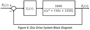
a) Consider the controller that we designed in tutorial:

Gc(s) = K_c = 12.14

Find the steady-state error to a ramp input with this controller. If we wish to reduce this error to 0.005, can we do it with a different K_c? (Hint: consider your stability limits!)

b) Well try a more complex controller of the form

G_c(s) = K_c(s + a)

which is sometimes called a proportional-derivative controller. Find the closed-loop transfer function, T(s) = P_o(s)/P_t(s).

c) Find the conditions (inequalities) on K_c and a such that the closed-loop system is stable. Use MATLAB to plot the stability boundaries (again, inequalities) on a K_c vs a plot.

d) Find values of K_c and a such that the steady-state error to a ramp is less than 0.005.

 Exercise 8: Using Root Locus

Consider the feedback control system in Figure 7. In this exercise, we'll walk through designing G_c(s) with different levels of complexity.

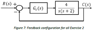
To this ends, do the following by hand (unless otherwise stated):

a) Sketch (by hand) the root locus and find the dosed loop poles when G_c(s) = K_c = 1. Also: find the steady-state error to a step and ramp inputs, ζ and the settling time.

b) In order to improve the transient response, a PD controller of the form

G_c(s) = K_c(s + a)

is being considered. Determine the values of K and a so that the closed loop system has an overshoot of 1.6 and a settling time of 2s for a step input. (Hint: use a to ensure that the poles are on the root locus). You may ignore the effect of the zero dynamics for this part.

c) What is the steady-state error to a ramp?

d) We now require that steady-state error to a ramp is eliminated. Your boss has told you to "just add an integrator" to the controller to eliminate the steady-state error. Sketch the root locus and use it to tell your boss why this won't work.

e) A smarter way to eliminate the steady-state error is to use a RID controller of the form

G_c(s) =  (K_c(s + a)(s + b)/s)

where a is the same as in b) and b is close to the origin. Select a suitable value for b so that the desired poles from b) are on the root locus. If necessary (it may or may not be!), adjust the value of K_c to ensure that the desired closed-loop poles are achieved. You may use MATIAB to check the location of the closed-loop poles.

f) Simulate the closed-loop step response in MATLAB using the PID controller from e). Twiddle K_c a and b (if necessary) to achieve your targets (i.e. 16% overshoot and a settling time of 2s).

Exercise 9: Lead-Lag design using Root Locus

Recall the disc drive problem from Tutorials, where we demonstrated that the open-loop system can be written as

We will now try to design a lead-lag compensator with the requirements that

• Overshoot ≤ 10
• T_s ≤ 75MS
• e_ramp(∞)≤ 0.001

Do the following (you may use MATLAB at your leisure, but be sure to explain your logic for your design choices):

a) Use MATLAB to draw the root locus when G_c = K_c.

b) Use MATLAB to draw the region where the dominant closed-loop poles must be to satisfy the transient requirements. Comment on your ability to achieve these requirements with a gain-only controller.

c) Design a lead compensator(s) to meet the transient requirements (i.e. overshoot and settling time).

d) Design a lag compensator to achieve the steady-state tracking requirement.

e) Use MATLAB to compute the resulting closed-loop poles and discuss second order dominance.

Some Hints:

• You may need to place more than one lead compensator for part c)
• When assessing second order dominance of the closed-loop system, be sure to cancel poles and zeros (i.e. use minreal).