Reference no: EM13733752

Part -1:

1)

a) the IS curve: lnYt= ln Y(t+1) -(1/O)rt

so the slope is: drt/dyt (is) = -O/Yt. That means that an increase in O will result in a steeper curve.

LM curve: Mt/Pt = Yt^(O/v) (1+rt / rt)^(1/v)

Ln(Mt/Pt) = (O/v) lnYt +(1/v)ln(1+rt) - (1/v)ln rt.

0 = (O/v)(1/Yt)dYt + (1/v)(1/(1+rt)) drt - (1/v)(1/rt)drt.

The slope is: drt/dyt (LM) = (Ort(1+rt))/Yt. That means that an increase in O will result in a steeper curve.

b) the curve IS is not affected by the value of V. while curve LM shifts upwards, since a decrease in v will result in an increase for the demand for real money.

c) IS is not affected byΓ(.)

optimal money holdings: BΓ'(Mt/Pt) = (it/(1+it)) U'(Ct)

B(Mt/Pt)^(-v) = (it/1+it) Yt^-O

Mt/Pt= B^(1/v) Yt^(O/v) (1+rt/rt)^(1/v)

So this means that the LM curve will shift downwards.

2)

a)AC= (PC/τ)+(αYPτ/2)i

∂AC/τ = -(PC/τ^2) + (αYP/2)I = 0

C/τ^2 = αYi/2

So τ*=(2C/αYi)^(1/2)

b)average real money holdings:M/P= αYτ/2

M/P = (αY/2) (2C/αYi)^(1/2)

M/P= (αCY/2i)^(1/2)

Ln(m/p) = (1/2)(lnα+lnY+lnC-ln2-lni)

(1/(M/P))(∂(M/P)/∂i) = -(1/2)(1/i)

Elasticity of real money with respect to i: (∂(M/P)/∂)(i/(M/P)) = -1/2

The elasticity with respect to Y : (∂(M/P)/∂Y)(Y/(M/P)) = ½

Average real money holdings increase in Y, and decrease in i.

3)

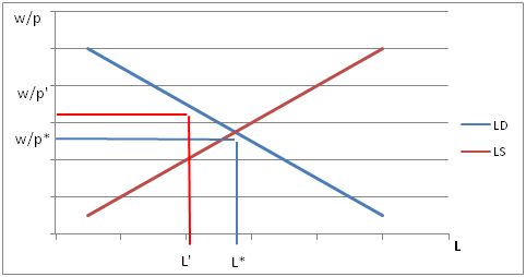
a) when p is at a level that generates maximum output, LS meets LD.

b) when p is above the level that generates maximum output, will cause unemployment.

4)

a)

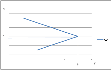
b)i)

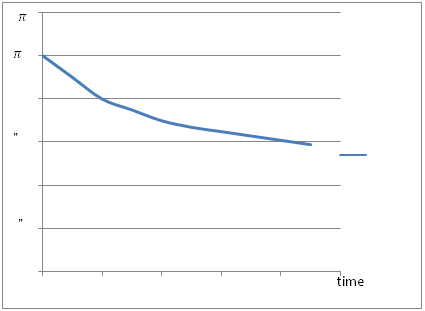
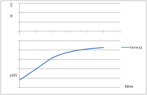
ii)

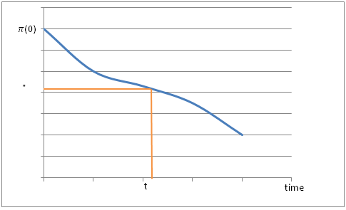
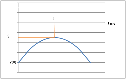
iii)

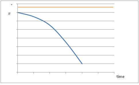
6)

a) the asset has an expected rate of return r. capital gain/loss plus dividends per unit time = rvp. There is no dividends per unit time while searching for the palm tree, and there is b probability per unit time of capital gain of (vc-vp)-c.  the difference in the price of the asset is(vc-vp) and -c is what the asset pays, so at the end we have rvp=b(vc-vp-c)

b) there is probability aL that a person will find another person with a coconut and trade with that person and gain u¯. the difference in the price of the asset is (vp-vc). So we end up with

rvp=al(vp-vc+u¯).

c)vp=(rvc/aL)+vc-u¯.

r((rvc/aL )+vc-u¯)= b(vc-(rvc/aL)-vc+u¯-c)

vc(r(r+aL+b))/aL = u¯(r+b)-bc

the value of being in state C: vc= (aL(u¯(r+b)-bc)) / r(r+aL+b)

the value of being in state p: vp= ((u¯(r+b)-bc)/(r+aL+b)) + (aL(u¯(r+b)-bc)/r(r+aL+b)) - u¯

so finally

vc-vp = (bc+u¯aL)/(r+aL+b).

e) vc-vp≥c

vc-vp = (bc+u¯a(b/a))/(r+a(b/a)+b) = (bc+bu¯)/(r+2b)

(bc+bu¯)/(r+2b) ≥ c

That means that

Bc+bu¯≥c  and   c(r+2b-b) ≤ bu¯

So finally we have

c≤ bu¯ / (r+b).

f) it is a steady-state equilibrium for no one who finds a tree to climb it for any value of c>0.

Yes there are values of c which there is more than one steady-state equilibrium for 0<c<bu¯/(r+b)

Yes, L = b/a has a higher welfare than L=0.  When L=0 people don't gain any utility since they don't climb a tree and don't have a chance to trade with other people and gain a coconut.

Part -2:

1. The stability of fiscal policy. (Blinder and Solow, 1973.) By definition, the budget deficit equals the rate of change of the amount of debt outstanding: δ(t) ≡ D ?(t). Define d(t) to be the ratio of debt to output: d(t) = D(t)/Y(t). Assume that Y(t) grows at a constant rate g > 0.

(a) Suppose that the deficit-to-output ratio is constant: δ(t)/Y(t) = a, where a > 0. ?

(i) Find an expression for d(t) in terms of a, g, and d(t).  ?

(ii) Sketch d(t) as a function of d(t). Is this system stable?

(b) Suppose that the ratio of the primary deficit to output is constant and equal to a > 0. Thus the total deficit at t, δ(t), is given by δ(t) = aY(t) + r(t)D(t), where r(t) is the interest rate at t. Assume that r is an increasing function of the debt-to-output ratio: r(t) = r(d(t)), where r′(•) > 0, r′′(•) > 0, limd→-∞ r(d) < g, limd→∞ r(d) > g.

(i) Find an expression for d(t) in terms of a, g, and d(t).  ?

(ii) Sketch d(t) as a function of d(t). In the case where a is sufficiently small that d ? is negative for some values of d, what are the stability properties of the system? What about the case where a is sufficiently large that d ? is positive for all values of d ?

2. Precautionary saving, non-lump-sum taxation, and Ricardian equivalence.

(Leland, 1968, and Barsky, Mankiw, and Zeldes, 1986.) Consider an individual who lives for two periods. The individual has no initial wealth and earns labor incomes of amounts Y1 and Y2 in the two periods. Y1 is known, but Y2 is random; assume for simplicity that E[Y2] = Y1. The government taxes income at rate τ1 in period 1 and τ2 in period 2. The individual can borrow and lend at a fixed interest rate, which for simplicity is assumed to be zero. Thus second-period consumption is C2 = (1 - τ1)Y1 - C1 + (1 - τ2)Y2. The individualchoosesC1 tomaximizeexpectedlifetimeutility,U(C1)+E[U(C2)].

(a) Find the first-order condition for C1.

(b) Show that E[C2] = C1 if Y2 is not random or if utility is quadratic.

(c) Show that if U ′′′(•) > 0 and Y2 is random, E[C2] > C1.

(d) Suppose that the government marginally lowers τ1 and raises τ2 by the same amount, so that its expected total revenue, τ1Y1 + τ2E[Y2], is un- changed. Implicitly differentiate the first-order condition in part (a) to find an expression for how C1 responds to this change.

(e) Show that C1 is unaffected by this change if Y2 is not random or if utility is quadratic.

(f) Show that C1 increases in response to this change if U ′′′(•) > 0 and Y2 is random.

3

Consider the Barro tax-smoothing model. Suppose that output, Y, and the real interest rate, r, are constant, and that the level of government debt out- standing at time 0 is zero. Suppose that there will be a temporary war from time 0 to time τ. Thus G(t) equals GH for 0 ≤ t ≤ τ, and equals GL there- after,whereGH >GL.Whatarethepathsoftaxes,T(t),andgovernmentdebt outstanding, D(t)?

4

Consider the Barro tax-smoothing model. Suppose there are two possible val- ues of G(t)-GH and GL-with GH > GL. Transitions between the two values follow Poisson processes (see Section 7.4). Specifically, if G equals GH, the probability per unit time that purchases fall to GL is a; if G equals GL, the probability per unit time that purchases rise to GH is b. Suppose also that output, Y, and the real interest rate, r, are constant and that distortion costs are quadratic.

(a) Derive expressions for taxes at a given time as a function of whether G equals  G H     or         G L ,    the            amount            of         debt     outstanding,    and      the       exogenous parameters. (Hint: Use dynamic programming, described in Section 10.4, to find an expression for the expected present value of the revenue the government must raise as a function of G, the amount of debt outstanding, and the exogenous parameters.)

(b) Discuss your results. What is the path of taxes during an interval when G equals GH? Why are taxes not constant during such an interval? What happens to taxes at a moment when G falls to GL? What is the path of taxes during an interval when G equals GL?

5.

Consider the Tabellini-Alesina model in the case where α can only take on the values 0 and 1. Suppose, however, that there are 3 periods. The period-1 median voter sets policy in periods 1 and 2, but in period 3 a new median voter sets policy. Assume that the period-1 median voter's α is 1, and that the probability that the period-3 median voter's α is 1 is π.

(a) Does M1 = M2?

(b ) Suppose that after choosing purchases in period 1, the period-1 median voter learns that the probability that the period-3 median voter's α will be1isnotπ butπ′,whereπ′ < π.Howdoesthisnewsaffecthisor her choice of purchases in period 2?

6. ThePersson-Svenssonmodel.(PerssonandSvensson,1989.)Suppose there are two periods. Government policy will be controlled by different policy- makers in the two periods. The objective function of the period-t policymaker is U + αt [V(G1) + V (G2)], where U is citizens' utility from their private consumption; αt is the weight that the period-t policymaker puts on public consumption; Gt is public consumption in period t; and V(•) satis- fiesV′(•)>0,V′′(•)<0.Privateutility,U,isgivenbyU =W-C(T1)-C(T2), where W is the endowment; Tt is taxes in period t; and C(•), the cost of raising revenue, satisfies C′(•) ≥ 1, C′′(•) > 0. All government debt must be paidoffattheendofperiod2.ThisimpliesT2 =G2+D,whereD=G1-T1 is the amount of government debt issued in period 1 and where the interest rate is assumed to equal zero.

(a) Find the first-order condition for the period-2 policymaker's choice of G2 given D. (Note: Throughout, assume that the solutions to the policy- makers' maximization problems are interior.)

(b) How does a change in D affect G2?

 (c) Think of the period-1 policymaker as choosing G1 and D. Find the first-

order condition for his or her choice of D.

(d) Show that if α1 is less than α2, the equilibrium involves inefficiently low taxation in period 1 relative to tax-smoothing (that is, that it has T1 < T2). Explain intuitively why this occurs.

(e) Does the result in part (d) imply that if α1 is less than α2, the period-1 policymaker necessarily runs a deficit? Explain.

Part -3:

1. Observational equivalence. (Sargent, 1976.) Suppose that the money supply isdeterminedbymt =c′zt-1 +et,wherecandzarevectorsandet isani.i.d. disturbance uncorrelated with zt-1. et is unpredictable and unobservable. Thus the expected component of m t is c ′ zt -1 , and the unexpected component is et. In setting the money supply, the Federal Reserve responds only to vari- ables that matter for real activity; that is, the variables in z directly affect y .

Now consider the following two models: (i ) Only unexpected money mat- ters,so yt = a′zt-1+bet+vt;(ii)allmoneymatters,so yt = α′zt-1+βmt +νt.In each specification, the disturbance is i.i.d. and uncorrelated with zt -1 and et.

(a) Is it possible to distinguish between these two theories? That is, given a candidate set of parameter values under, say, model (i), are there param- eter values under model (ii ) that have the same predictions? Explain.

(b) Suppose that the Federal Reserve also responds to some variables that donotdirectlyaffectoutput;thatis,supposemt =c′zt-1+γ′wt-1+et and that models (i) and (ii) are as before (with their distubances now uncorrelated with wt -1 as well as with zt -1 and et). In this case, is it pos- sible to distinguish between the two theories? Explain.

2. Consider an economy consisting of some firms with flexible prices and some with rigid prices. Let pf denote the price set by a representative flexible-price firm and pr the price set by a representative rigid-price firm. Flexible-price firms set their prices after m is known; rigid-price firms set their prices be- fore m is known. Thus flexible-price firms set pf      = pi∗ = (1 - φ)p + φm, and rigid-price firms set pr = Epi∗ = (1 - φ)Ep + φEm, where E denotes the expectation of a variable as of when the rigid-price firms set their prices.

Assume that fraction q of firms have rigid prices, so that p = qpr+ (1-q)pf.

(a) (b) (c)

Find pf in terms of pr,m, and the parameters of the model (φ and q). Find pr in terms of Em and the parameters of the model.

(i ) Do anticipated changes in m (that is, changes that are expected as of when rigid-price firms set their prices) affect y ? Why or why not?

(ii ) Do unanticipated changes in m affect y ? Why or why not?