Reference no: EM133133835

FE 621 Computational Methods in Finance - Stevens Institute of Technology

Problem 1. Barrier options.

The purpose of this problem is to compute the price of an up-and-out put option. An up-and-out put option (UOP) with strike K and barrier level H has the same payoff at time T as a vanilla put option, (K S_T)⁺, unless the stock price goes above the barrier level H during the life of the option, in which case the holder receives nothing.

(a) Is such an option cheaper or more expensive than a vanilla put option? Explain.

(b) The price of an UOP option is given by

P = e^-rTE[(K - S_T)⁺1{sup_t≤T S_t ≤ H}].

The standard Monte Carlo estimator for the price is given by

Pˆ_n,m = e^-rT 1/n Σⁿ_k=1 (K - S_m(k))⁺1{sup_t≤T St ≤ H}

where ti = T/m and (Sˆ₁(k), . . . , Sˆ_m(k)) is the k-th simulated path of GBM at times (ti)_1≤i≤m.

Is the estimator Pˆ_n,m biased? Is it biased low or high? Explain.

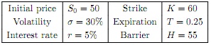
(c) Use the parameters in the table below to compute an estimate of the price using (0.1) along with a 95% confidence interval. Use m = 63 and n equal to at least 100, 000.

 

(d) An UOP with a rebate pays its holder a rebate R when the option is knocked out (i.e. when it hits the barrier). Explain carefully how you would extend the Monte Carlo estimator (0.1) to handle the case with a rebate.

(e) Use your estimator in part (d) to compute an estimate of the price an UOP with a rebate together with a 95% confidence interval. Use the same parameters as in (c) and set the rebate to R = $5.

Problem 2. Reduction of the bias.

For a geometric Brownian motion (S_t)_t≥0 and x, y < H we have the following formula:

p(ti, x, ti+1, y) = P(sup       S_u ≥ H|S_ti = x,S_ti+1 = y) = exp (2/σ²/(t_i+1 - t_i)ln(H/x)ln(y/H))
                          t_i≤u≤t_i+1

The above formula gives the probability that the barrier H was crossed between times ti and ti+1, given that the price was x at time ti and y at time ti+1. We can use this result to improve the estimators in Problem 1.

(a) An unbiased estimator for the price that improves (0.1) is given by

P˜ = e^-rT 1/n Σⁿ_k=1(K - Sˆ_m (k))+.1 - q(0, S₀, T, S_mˆ (k)).

Use this estimator to give an estimate of the UOP option price with a 95% confidence interval. Is it different from the interval in Problem 1(c)?

Extra credit: Show formally that the estimator is unbiased. That is, show E[P^~n,m] = P.

(b) Use the barrier crossing formula (0.2) to construct an estimator for the price of an UOP option with a rebate that improves the estimator in Problem 1(d). Clearly explain your simulation procedure.

Use your estimator to given an estimate of the rebate option price and a 95% confidence interval. Is it different from the interval in Problem 1(e)?

(c) Let us now suppose that the stock price follows the CEV model,

dS_t = rdt + αS_t^β-1dW_t.

For an UOP without rebate, one can use the estimator in Problem 1(a). The only difference is that the stock price paths have to be simulated step by step using the Euler discretization scheme.

Explain clearly how the barrier crossing formula (0.2) can be used to improve this estimator.

In this part you only need to explain your simulation procedure - you do not have to implement your algorithm or provide any numerical estimates.

Problem 3. Asian options.

A continuously sampled Asian option with maturity T has payoff

(A_T - K)⁺ = (1/T∫₀^TSudu - K)⁺

Assume that (S_t)_t≥0 follows a GBM and let t_i = iT/m = iΔt. The quantity A_T cannot be simulated exactly so we consider two different approximations:

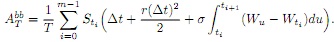
(i) First, A_T can be approximated by a Riemann sum (r stands for Riemann):

A^r_T = 1/m ∑^m-1_i=0 S_ti

To simulate A^r_T one can simulate (W_t1 , . . . , W_tm) and then use those values to compute (S_t1 , . . . , S_tm ).

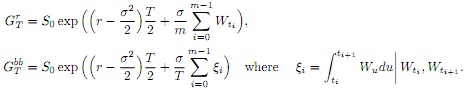
(ii) Second, A_T can be approximated using the following expression (bb stands for Brownian bridge):

 

Using properties of Brownian motion one can show that

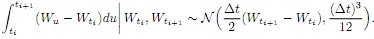
It follows that to simulate A_T^bb one can first simulate (W_t1 , . . . , W_ti) and then, conditionally on those values, simulate the integrals ∫_ti^ti+1 (W_u - W_ti)du.

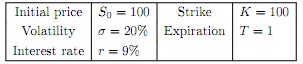
Using the approximations A_T^r and A_T^bb, give estimates for the price of the Asian option. Use the parameters in the table below. Take m = 10, 50, 100 and n = 50, 000. Give 95% confidence intervals and present your results in a table.

 

Problem 4. Variance reduction using control variates.

Let G = exp (1/T ₀∫^T ln(S_u)du)² In this problem we use the option with payoff (G_T - K)⁺ as a control variate to reduce the variance of the estimators in Problem 3.

(a) Show that E[e^-rT (G_T - K)⁺] can be computed using the Black-Scholes formula using the following parameters:

(b) The quantity G_T cannot be simulated exactly but it can be approximated in the following ways:

 

Importantly, the random variables used to simulate A_T^r or A_T^bb can also be used to simulate G_T^r and G_T^bb.

To use G_T^r and G_T^bb as control variates, we need explicit expressions for E[e^-rT (G_T^r -K)⁺] and E[e^-rT (G_t^bb -K)⁺].

However, in this problem we will simply use the formula in part (a) for E[e^-rT (G_t^T - K)⁺] as an approximation for those values.

Compute Monte Carlo price estimates and 95% confidence intervals for the option in Problem 3 using control variates. Use G_T^r as a control variate for A_T^r and G_T^bb as a control variate for A_T^bb.

Use same values of m and n as before and present your results in a table. Also report your estimates for the control variate slope b∗.

How to the price estimates and confidence intervals deviate from those in Problem 3?

Does using Abb and Gbb rather than Ar and Gr seem to be worth the additional complexity?

Problem 5. Bond pricing.

In the Vasicek model, the short rate under the risk-neutral measure has dynamics

 

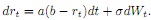
For this process it can be shown that

 

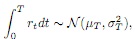
where the mean and variance are given by

(a) The price at time 0 of a zero coupon bond with maturity T is

B (T) = E[e^-0∫Trtdt

Use (0.3) to give an explicit expression for the price B₀(T).

(b) Suppose that a = 0.25, b = 0.04, σ = 0.1, r0 = 0.05, and T = 1. Price the bond in (a) using Monte Carlo with Euler discretization to simulate (rt)t≥0. Provide a 95% confidence interval of width less than 1 cent.

(c) Analyze the bias and variance of your estimator in (b).

Hint: Plot the bias as a function of m for m between 5 and 52 (and a fixed large value of n). Plot the standard deviation as a function of n (for a fixed large value of m). You may also want to consider log-log plots.

(d) Are your results in (c) in line with theoretical results about the order of bias and variance in Monte Carlo simulations?

Problem 6. Portfolio wealth growth.

Consider a portfolio with initial value X(0) = 1. Between times t-1 and t the value of the portfolio is multiplied by a random factor r(t) given by

 

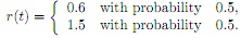
That is, the value X(t) at time t is given by r(t)XQ(t - 1) where X(t - 1) is the value at time t - 1. More generally,

(a) Use Monte Carlo simulation to estimate the expected portfolio value E[X(t)] for t between 1 and 50. Use n = 100, 000 simulations and plot your results.

Based on this, would you consider the portfolio a favorable investment option?

Note: You can also use E[r(i)] = 0.5 0.6 + 0.5 1.5 = 1.05 to obtain E[X(t)] = X(0) 1.05n. Display this closed-form result for E[X(t)] with your Monte Carlo estimates.

(b) Visualize a few wealth trajectories between time 0 and time 50. That is, visualize independent simulations of the wealth sequence X(0), X(1), . . . , X(50).

What do you observe? Based on this, would you consider the portfolio a favorable investment option?

(c) Can you explain the apparent discrepancy between the results in (a) and (b)?