Reference no: EM13752833

Question 1.

a. You run the following two models through OLS and record the R²:

Model A: y = β₀ + β₁x₁ + β₂x₂ + u → R²_A

Model B: y = β₀ + β₁x₁ + β₂x₂ + β₃x₃ + u → R²_B

Which is true: R²_A ≥ R²_B or R²_A ≤  R²_B? Give a one sentence explanation.

b. True or False: The homoskedasticity assumption is required for OLS estimates to be unbiased.

c. You estimate the following model using a sample of 100 observations.

y = β₀ + β₁x₁ + β₂x₂ + β₃x₃

How many degrees of freedom does this model have? You must show your math.

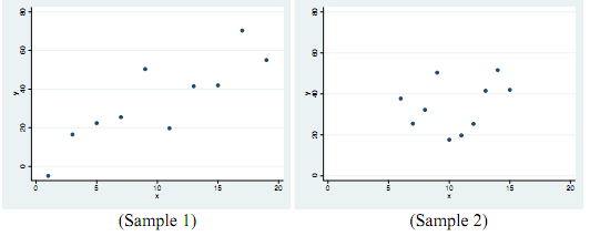
Question 2. The following random samples of 10 observations were taken from the same population. You estimate the slope and intercept of the following model twice, once using each sample:

y = β₀ + β₁x + u

Which sample do you think would yield a slope estimate with a smaller standard error? (In other words for which sample will se(β₁) be smaller, or alternatively, for which sample would you be most sure about your estimated slope?). Explain briefly.

HINT: While not necessary, it may help to think if you can say anything definitive about any of the ingredients in the numerator & denominator of the formula for the standard error:

se(β^{^}₁) = σ^{^}/√SSTx where σ^{^} = √SSR/n-2 = √(1/n-2)(_i=1Σⁿ u^{^}_i²), SSTx = _i=1Σⁿ (x_i -x^- )²

Question 3. On average a baby born with a low birth weight is more likely to have health problems. According to the Centers for Disease Control (CDC): "Smoking during pregnancy can cause a baby to be born too early or to have low birth weight."

Suppose you are trying to uncover the relationship between the number of cigarettes smoked per day by pregnant mothers and the birth weight of their babies.

a. Use the dataset called PS2_BWGHT.dta to regress birth weight (variable bwght) against the number of cigarettes smoked per day (variable cigs):

bwght = β₀ + β₁cigs + v

The results follow the sample regression line: bwght^- = β^-₀ + β^-₁cigs + v

To do this in STATA, use the following command:

regress bwght cigs.

What is the interpretation of β₁, the estimated coefficient on cigs that you calculated with STATA? [HINT: Use the describe command to find out the units of the two variables]

b. Do you think the zero conditional mean assumption is satisfied in the model that was estimated in part (a)? In other words, does (v|cigs) = E(v) = 0? Explain in 2-3 sentences.

c. Family income is a factor that we omitted from the model in part (a). The model should have been:

bwght = β₀ + β₁cigs + β₂faminc + u

In part (a) we omitted this relevant variable. Do you think this resulted in the estimate of !! in part (a) being biased? If so, in what direction do you think it was biased? [HINT: Use the table on the bottom of page 90 that we discussed in class]

d. EXTRA CREDIT. Luckily, family income is in the dataset. Try running the model controlling for family income. How does the new estimated coefficient on cigs differ from what you calculated in part (a), and does this agree with your prediction in part (c)?

Question 4. In a study relating college grade point average to time spent in various activities, you distribute a survey to several students. The students are asked how many hours they spend each week in four activities: studying, sleeping, working, and leisure. Any activity is put into one of four categories, so that for each student, the sum of hours in the four activities must be 168 (total number of hours in a week).

a. In the following model:

GPA = β₀ + β₁study + β₂sleep + β₃work + β₄leisure + u

does it make sense to hold sleep, work, and leisure fixed, while changing study?

b. Explain why this model violates the No perfect collinearity assumption for unbiasedness. (Hint: Remember perfect collinearity can happen when one independent variable is a linear combination of one or more of the other independent variables)

Question 5. Suppose you are trying to uncover the relationship between education and wages, where education is measured with years of school completed and wage is measured by hourly wage. You know the population model is:

wage = β₀ + β₁school + β₂ttl_exp

wage = hourly wage

school = years of schooling completed

ttl_exp = total years of work experience

a. Using the dataset nlsw_ps2.dta you run the model specified above. To do this in Stata run the following command after the dataset has been opened in the program:

regress wage school ttl_exp

Report output. What is the interpretation of the estimated β^₁?

b. What if your dataset didn't have a measure for total work experience so instead you ran this model:

wage = β₀ + β₁school

and obtained estimates β'₀ and β'₁. Would you expect β'₁ to be biased? If so, in what direction would you expect the bias to be? Show your work.

Instructions for opening an external dataset in Stata.

If you are using a copy of Stata that is installed locally (like in a UIC lab), follow the following procedure to open the dataset:

1. Download the file from blackboard and save to your desktop.

2. Open Stata

3. In Stata, go to File, Open, and double click the downloaded file

If you are using a copy of Stata that you purchased from the UIC Webstore follow the following procedure to open the dataset:

1. Download the file from blackboard and save to your desktop.

2. Right click and copy the downloaded .dta or .do file

3. Open Stata

4. In Stata, go to File, Open, and create a new folder

5. Paste the file into the new folder, double click the file and it should open up.

Attachment:- data.rar