Reference no: EM132654472

Question 1: In studying the purchase of durable goods Y(Y = 1 if purchased, Y = 0 if no purchase) as a function of several variables for a total of 762 house¬holds, Janet A. Fisher' obtained the following LPM results:

Explanatory variable	Coefficient	Standard error
Constant	0.1411
1957 disposable income, X1	0.0251	0.0118
(Disposable income        X1)2, X2	-0.0004	0.0004
Checking accounts, X3	-0.0051	0.0- 08
Savings accounts, X4	0.0013	0.0047
U.S. Savings Bonds, Xs	-0.0079	0.0067
Housing status: rent, Xs	-0.0469	0.0937
Housing status: own, X7	0.0136	0.0712
Monthly rent, X8	-0.7540	1.0983
Monthly mortgage payments, X9	-0.9809	0.5162
Personal noninstallment debt, X10	-0.0367	0.0326
Age, Xii	0.0046	0.0084
Age squared, X12	-0.000'	0.0001
Marital status, X13 CI = married)	0.1760	0.0501
Number of children, X14	0.0398	0.0358
(Number of children = X14)2, X1-5	-0.0036	0.0072
Purchase plans, X16 1 = planned; 0 otherwise)	0.1760	0.0384

a. Comment generally on the fit of the equation.
b. How would you interpret the coefficient of -0.0051 attached to checking account variable? How would you rationalize the negative sign for this variable?
c. What is the rationale behind introducing the age-squared and number of children-squared variables? Why is the sign negative in both cases?
d. Assuming values of zero for all but the income variable, find out the conditional probability of a household whose income is $20,000 purchasing a durable good.
e Estimate the conditional probability of owning durable good(s), given: X1= $15,000, = $3000, X4 = y 5 000, X6 = 0 , X7 = 1, Xg = $500, X9 = $300, X10 = 0, X11 = 35, X13 = 1, X14 = 2, X16 = 0.

Question 2: From the household budget survey of 1980 of the Dutch Central Bureau of Statistics, J. S. Cramer obtained the following logit model based on a sample of 2820 households. (The results given here are based on the method of maximum likelihood and are after the third iteration)** The purpose of the logit model was to determine car ownership as a function of (logarithm of) income. Car ownership was a binary variable: Y= 1 if a household owns a car, zero otherwise.

^{^}L_i= -2.77231 + 0.347582 In Income
t = (-3.35) (4.05)
x²(1 df) = 16.681 (p value = 0.0000)

where ^{^}L_i estimated logit and where In Income is the logarithm of income. The x2 measures the goodness of fit of the model.

a. Interpret the estimated logit model.
b. From the estimated logit model, how would you obtain the expres-sion for the probability of car ownership?
c. What is the probability that a household with an income of 20,000 will own a car? And at an income level of 25,000? What is the rate of change of probability at the income level of 20,000?
d. Comment on the statistical significance of the estimated logit model.

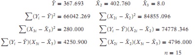
Question 3: From the following data estimate the partial regression coefficients, their standard errors, and the adjusted and unadjusted IV values:

Question 4: In a multiple regression model you are told that the error term ui has the following probability distribution, namely ui ~ N(0, 4). How would you set up a ANome Garbo experiment to verify that the true variance is in fact 4?

Question 5: Show that r²1,2,3 = (R² - r²13)/( 1 - r²13) and interpret the equation.

Question 6: If the relation at α1X1 + α2X2 + α3X3 = 0 holds true for all values of X1, X2, and X3, find the values of the three partial correlation coefficients.

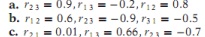
Question 7: Is it possible to obtain the following from a set of data?

Question  8: Consider the following model

Yi = β1 + β2 Educations + β2 Yeats of experience + ui
Suppose you leave out the years of experience variable. What kinds of problems or biases would you expect? Explain verbally

Question 9: Show that β2 and β3 in (7.9.2) do, in fact, give output elasticities of labor and capital. (This question can be answered without using calculus-,. just recall the definition of the elasticity coefficient and remember that a change in the logarithm of a variable is a relative change, assuming the changes are rather small.)

Question 10: Consider the three-variable linear regression model discussed in this chapter.

a. Suppose you multiply all the X2 values by 1 What will be the effect of this rescaling, if any on the estimates of the parameters and their stan-dard errors?
b Now instead of a, suppose you multiply all the Yvalues by 2. What will be the effect of this, if any on the estimated parameters and their stan-dard errors?

Question 11: A researcher is using data for a sample of 88 houses sold in an urban area during a recent year to investigate the relationship between house prices Yi (measured in thousands of dollars) and house size Xi (measured in square meters). Preliminary an4ysis of the sample data produces the following sample information:

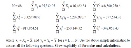
(a) Use the above information to compute OLS estimates of the intercept coefficient β1 andthe slope coefficient β2
(b) Calculate an estimate of σ2, the error variance.
(c) Compute the value of R2, the coefficient of determination for the estimated OLS
sample regression equation. Briefly explain what the calculated value of R2means.
(d) Perform a test of the null hypothesis H0: β2 = 0 against the alternative hypothesis H1:β2 ≠ 0 at the 5% significance level (i.e., for significance level α = 0.05). Show how youcalculated the test statistic. State the decision rule you use, and the inference you woulddraw from the test. Briefly explain what the test outcome means.