Reference no: EM132274578

Assignment -

The purpose of this assignment is threefold. First, it illustrates some stylized facts on return predictability. Second, want to highlight the connection between theory and empirics (e.g., cointegration). Third, in order to achieve the previous point, going to walk you step-by-step through the theory so that you will become familiar with an important tool from the asset pricing literature, the Campbell-Shiller decomposition.

1. Dividend-price ratio

From the literature it is known that the dividend-price ratio (a.k.a. the dividend yield) has some predictive power for future returns (e.g., Fama and French (1988)).

(a) Having prepared the time series for the excess return (R^e_t) and the dividend-price (D_t/P_t), you are now ready to run "predictive regressions".

Estimate a simple univariate regression with the excess return in year t + 1 as the dependent and the dividend-price ratio in year t as the independent variable, i.e., run the following regression:

R^e_t+1 = α + β (D_t/P_t) + u_t+1.

Extend your analysis from the one-year horizon to the five-year horizon. In order to calculate the cumulative excess return, R^e,cum_t+5, cumulate the gross return (including dividends) on the stock market index over the next five years and subtract from this the cumulative gross return on the three month U.S. Treasury bill over the same time span, i.e., determine

R^e,cum_t+5 = _j=1Π⁵(1 + R_t+j) - _j=1Π⁵(1 + R^f_t+j).

Use the dividend-price ratio in year t as the independent variable and the cumulative excess return in year t+5 as the dependent variable, i.e., run the following regression:

R^e,cum_t+5 = α + β (D_t/P_t) + u_t+5.

For each regression, report the parameter estimate for β, the corresponding t-statistic, and the R². Based on a 5% significance level, discuss the statistical significance and the economic significance of your results. Do you think the R² is a good measure of economic significance for explaining variation in expected returns?

(b) Campbell and Shiller (1988) provide one way, to understand the result from exercise part (a). In their seminal paper, the authors derive the "Campbell-Shiller decomposition" based on the following steps (steps are in attached file).

In contrast to Campbell and Shiller (1988) who work with the log price-dividend ratio, we are interested in the log dividend-price ratio, so the previous Equations (4), (5), and (7) (equations are attached) become:

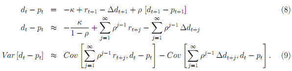
How large are the two right-hand side components of Equation (9), i.e., how large is the long-run impact of log returns and log dividend growth on the variation in the log dividend-price ratio?

Before you can look into this, you have to calculate the dividend growth for which the following transformation might be useful:

(D_t+1/P_t+1)/(D_t/P_t) (P_t+1/P_t) = D_t+1/D_t.

Start your analysis by running three simple regressions for a forecast horizon of one year. In all three regressions, use the log dividend-price ratio in year t as the independent variable. As the dependent variable, use the log return in year t + 1 in the first equation, the log growth rate of the dividend in year t + 1 in the second, and the log dividend-price ratio in year t + 1 in the third regression. Run the following regressions.

r_t+1 = α_r + β_r (d_t - p_t) + u^r_t+1

Δd_t+1 = α_d + β_d(d_t - p_t) + u^d_t+1

d_t+1 - p_t+1 = α_Φ + Φ(d_t - p_t) + u^dp_t+1.

For each regression, report the parameter estimate for the slope coefficient, the corresponding t-statistic, and the R².

(c) Assume in the following that ρ = 0.96. Taking a look at Equation (8), ignoring the constant κ, regressing both sides on d_t - p_t, and solving for β_r implies the following connection between the parameter estimates you just calculated.

1 ≈ β_r - β_d + ρΦ

β_r ≈ 1 - ρΦ + β_d. (10)

Consequently, we cannot form the null hypothesis that β_r = 0 without changing β_d or Φ. In particular, as long as Φ is non-explosive (i.e., Φ < 1/ρ ≈ 1/0.96 ≈ 1.04), we cannot choose a null hypothesis in which both dividend growth and returns are not forecastable (i.e., β_r = 0 and β_d = 0). To generate a coherent null hypothesis with β_r = 0, we must assume a negative β_d, and then address the absence of this negative β_d in the data.

Therefore, the next step of your analysis is to divide both sides of Equation (9) by Var [d_t - p_t] which allows us to express its two right hand side components in terms of the regression coefficient β (y, x) = Cov[y, x]/Var[x]:

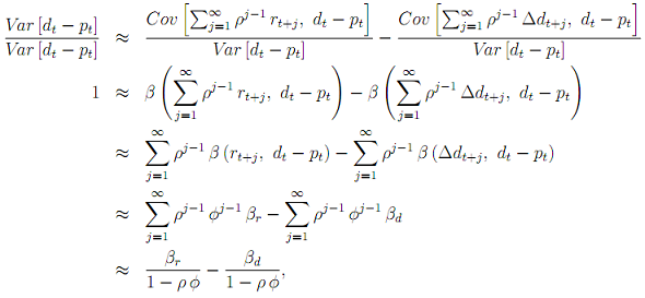
where the last step follows from taking the sum of an infinite geometric series. In order to make sure that the above equation holds exactly, we have to adjust it slightly:

1 = β^{^}_r/(1 - ρΦ^{^}_implied) - β^{^}_d/(1 - ρΦ^{^}_implied). (11)

where Φ^{^}_implied = 1/ρ (1 - β^{^}_r + β^{^}_d) which follows from solving Equation (10) for Φ. Calculate the two coefficients shown in Equation (11). Try to connect the different pieces of the puzzle you took a look at over the course of this exercise and explain what you have learned about return predictability.

2. Consumption-wealth ratio

(a) Check the three time series for consumption, financial wealth, and labor income for stationarity. Perform an Augmented Dickey Fuller (ADF) test with up to 12 lags and determine the optimal lag length p using Schwarz's Bayesian information criterion. As alternative model, select an AR(p) model with drift, but without a time trend. Report the p-value for each test and provide an economic interpretation of your results using a significance level of 5%.

(b) To eliminate potential concerns about endogeneity between the right-hand side variables, you decide to add leads and lags of the first differenced variables a and y to the standard regression. Hence, you want to estimate the following model (using OLS):

c_n,t = α + β_aa_t + β_yy_t + _s=-8∑⁸ b_a,sΔa_t-s + _s=-8∑⁸b_y,sΔy_t-s + u_t,

where Δ denotes the first difference operator. Report the values of estimated coefficients β^{^}_a and β^{^}_y. Use those results to estimated (cay)^{^}_t = c_n,t - β^{^}_a a_t - β^{^}_y y_t,  i.e.,d (cay)^{^}_t represents the estimated residuals (u^{^}_t) including the estimated intercept (α^{^}) (we ignore the first difference terms in the following). Use the first step of the Engle-Granger two-step method to test (cay)^{^}_t for cointegration. Report the p-value and provide an economic interpretation of your results using a significance level of 5%.

(c) Since you are worried about the number of cointegrating relations between the three variables, you run a Johansen test. Focus on the time series c_n,t, a_t, and y_t (ignore all the first difference terms in the previous exercise part). Use two lags, and specify that the model under the null hypothesis contains an intercept, but no trend. Under the alternative hypothesis, specify that the model contains neither an intercept nor a trend. Report the p-values for the two test statistics for r = 0, 1, 2 and provide an economic interpretation of your results using a significance level of 5%.

(d) Estimate the following vector error correction model (which can also be considered as three separate error correction models):

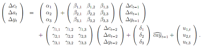
Report the parameter estimates ford (cay)^{^}_t-1, the corresponding t-statistics, and the R² for each equation. Based on a significance level of 5%, provide an economic interpretation of your results.

(e) Finally, you want to check whether (cay)^{^} can predict returns on the U.S. stock market index. Estimate a simple univariate regression with the log return in quarter t + 1 as the dependent and (cay)^{^} in quarter t as the independent variable, i.e., run the following regression:

r_t+1 = α + β(cay)^{^}_t + u_t+1.

Report the parameter estimate for β, the corresponding t-statistic, and the R². Based on a significance level of 5%, provide an assessment of the statistical and economic significance of your results. Try to connect the different pieces of the puzzle you have taken a look at over the course of this exercise and explain what you have learned about return predictability.

3. Dividend-price ratio & consumption-wealth ratio

You are interested in the similarities and differences between the dividend-price ratio (dp_t) and the consumption-wealth ratio (cay_t). Do both of them capture the same variation or something different? Put differently, if you run a regression using both of them, will both turn out to be significant, or will one become insignificant? In order to answer these questions, you want to perform a horserace between dp_t and cay_t.

Download the data set "assignment2 task3 data.xlsx". It contains (from left to right column) the following annual time series:

• Ret_d: the simple net return on the U.S. stock market index including dividends,
• Ret_x: the simple net return on the U.S. stock market index excluding dividends, and
• cay: the log (aggregate) consumption-wealth ratio.

Note that the sample length is different from the first task. Calculate the log return (r_t), the log dividend growth (Δd_t), and the log dividend-price ratio (d_t - p_t) as described previously. Run the following regressions:

r_t+1 = α₁ + β_1,1 (d_t - p_t) + β_1,2cay_t + u^r_t+1

Δd_t+1 = α₂ + β_2,1 (d_t - p_t) + β_2,2cay_t + u^d_t+1

d_t+1 - p_t+1 = α₃ + β_3,1 (d_t - p_t) + β_3,2cay_t + u^dp_t+1

cay_t+1 = α₄ + β_4,1 (d_t - p_t) + β_4,2cay_t + u^cay_t+1

For each regression, report the parameter estimates for β, the corresponding t-statistics, and the R². Based on a significance level of 5%, provide an economic interpretation of your results.

Attachment:- Assignment File.rar