Reference no: EM132381234

ENS6160: SIGNALS & SYSTEMS ASSIGNMENT 2

Analysing a simple system

Condition monitoring of equipment is an essential part of modern predictive maintenance. This involves the measuring of various parameters of the equipment (e.g. temperature, vibration) to identify significant changes that could indicate impending failure. Preventive maintenance based on such indicators can prevent catastrophic failure and consequent impacts (financial loss, injury or even death).

Vibration sensors convert mechanical vibrations detected into electrical signals that can then be sent to condition monitoring systems that process the signals to extract signal features (both time domain and frequency domain features). This data can then be analysed to determine if equipment requires attention (de Silva, 2007).

Accelerometers are dynamic sensors commonly used in vibration sensors. Piezoelectric accelerometers are extensively used as vibration sensors due to their light weight and high- frequency response (de Silva, 2007).

The basic principle of operation behind a piezoelectric accelerometer is the displacement of a small inertial mass on a piezoelectric crystal and restrained by a stiff spring. Consistent with Newton's second law of motion (F = ma), as an acceleration is applied to the device, a force develops which displaces the mass. Movement of the inertial mass distorts the piezoelectric crystal, changing the output signal voltage. The fluid (usually air) trapped inside the device acts as a damper, resulting in a second order lumped physical system.

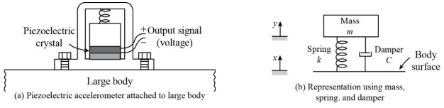
Figure 1: Piezoelectric accelerometer components and lumped physical model

In this figure:
• x is the position of the large body, with its rest position given by x = 0.
• The mass m represents the inertial mass within the accelerometer.
• The height of mass m above its reference level is called y. The reference level is chosen such that when accelerometer is at rest, y = 0.
• The voltage output, V, would be proportional to the change in the difference between x
and y due to piezoelectric effect.

Section 1: Mathematical Analysis of System

1. Draw a free-body diagram showing all the forces acting on the inertial mass m shown in Figure 1(b).

2. Let z(t) = y(t) - x(t) . From the earlier description, diagrams and the laws of Physics, show that the motion of the accelerometer can be described by the LCCDE (linear constant- coefficient differential equation) below:

d²z(t)/dt² + C/m dz(t)/dt + k/m z(t) = - d²x/dt²

Equation (1) shows that the output response depends on the acceleration of the large body.

3. Using the Laplace transform of the equation above, find an expression for H(s) , the system transfer function, taking z(t) as the system output.

The accelerometer is a damped second order system. It is common to express the homogenous second order DE for such a damped system as

d²z(t)/dt²  + 2Çω_n dz(t)/dt + ω²_nz(t) = 0                      (2)

where Ç is the damping ratio and ω_n is the undamped natural (resonant) frequency.

4. From equations (1) and (2), determine expressions for Ç (the damping ratio) and ω_n (the natural frequency) in terms of the parameters m, k and C

5. Determine the characteristic equation and eigenvalues (characteristic values) for this system based on equation (2) above (in terms of ω_n and Ç ).

6. From the answer to part 5, determine the full mathematical expression (in terms of ω_n and
Ç ) for the natural response of the system for the following cases:
a. Ç = 0
b. 0 < Ç < 1
c. Ç = 1
d. Ç > 1

Consider an accelerometer with the following parameters:
m = 4.8 x 10^-5 kg
k = 800 N/m

7. Determine ω_n (in rad/s) for this vibration sensor and the corresponding value for f_n (in Hz).

8. Calculate the required value of C in order to achieve Ç = 1

Section 2: System analysis using Matlab

In this section, the system responses should be analysed using Matlab. Refer to the document "A Brief MATLAB Guide" in order to understand how to represent LTI systems in Matlab, and hence how to determine impulse response, step response and frequency response of systems. Sample Matlab code that has been provided as part of learning materials can also be modified to suit. Students are advised to refer to the help function within Matlab as well as online Matlab documentation for more details. Note: MATLAB is installed in the engineering computer labs.

Using the commands given in the Guide, analyse the response of the vibration sensor using the m and k parameters given in Section 1 and C value calculated in question 8:

9. Plot the impulse response and step response of the system for 0.01 seconds duration and time ‘step size' of 10 nanoseconds (1e-8 sec) using the impulse and step functions. Include all plots (properly labelled) in your submission.

10. Determine the frequency response from 1000 to 10⁶ rad/s using the freqs command. Plot the magnitude and phase response over this frequency range. Hint: Use frequency ‘step size' of 10 rad/s.

Hint 1: You can plot all 4 graphs in one go using a 2 x 2 matrix of plots using subplot(22n), where n determines which of the 4 subplots gets used.

Hint 2: In order to clearly see variations over a range of frequencies, it is best to use a log scale for the frequency and magnitude (phase would still be displayed using linear scale). The functions loglog (for magnitude) and semilogx (for phase) can be used instead of plot.

11. Determine the magnitude response at mn. Determine the frequency of the -3dB point (where magnitude = 1⁄√2). Hint: Use the ‘data cursor' tool on the plot of the magnitude response. It shows the x and y values of the plot as you move along the curve.

12. Discuss the response of the system. Why do the impulse and step responses have that particular shape? How well will this accelerometer fulfil its purpose of a vibration sensor? Based on the frequency response, what limitations will there be on its usefulness?

Note: The function of a vibration sensor is to provide an accurate measurement of vibrations over a range of frequencies.

13. Repeat the analysis above (steps 9 - 11) for the following damping ratios

a. Ç = 0.3

b. Ç = 0.5

c. Ç = 0.7

d. Ç = 1.5

e. Ç = 2.0

Hint 3: It would be more efficient to put all the necessary commands into a script file (a .m file) so you can edit the parameters and then run all the commands at once.

14. Based on the results of the Matlab analysis above, which of the 6 values of damping ratio tested would be best for a vibration sensor. Clearly justify your selection and relate your selection to a sample application where appropriate.

Section 3: Modelling system response to input and effectiveness

The vibration sensor modelled previously (using the Ç value chosen in the previous step) is to be used on a pump designed to run at 1800 rpm. The vibration output of the pump during normal operation can be modelled by a sinusoid of that frequency (30Hz).

The M-file for the custom-written function inputsig has been provided, with explanatory comments in the file.

15. Use the inputsig function to generate a sinusoid of 30 Hz with magnitude 1 and appropriate duration, then simulate the sensor response to this function and plot both the input and output response vs time.

Hint 4: The system response to an input signal can be simulated using the lsim function. Following is some sample code that shows how this function could be used.
[xsig, t1] = inputsig(0.1); % generate signal duration 0.1
Sys1 = tf(B,A); % define system, use tf (transfer function) Sysout = lsim(Sys1, xsig, t1); % simulate LTI system response

Note: Students are advised to refer to the help function within Matlab as well as the online Matlab documentation for more details.

16. Repeat step 15 with the input signal being (a) square wave and (b) pulse

17. Compare the system response to the 3 types of input and explain the output signal for each and the differences.

Failing parts in rotating mechanical devices often produce non-sinusoidal vibrations (e.g. pulses or square waves) at the same frequency as the normal rotating frequency.

18. Repeat the simulation in step 15 with a combination of a sinusoid of amplitude 1 and a square wave of amplitude 0.1. Describe any visible differences in input and output waveforms due to the addition of the square wave. Hence comment on the suitability of using the vibration sensor to detect faults in the system.

19. Repeat the simulation in step 18 with a combination of a sinusoid of amplitude 1 and a pulse wave of amplitude 0.1. Describe any visible differences in input and output waveforms due to the addition of the pulse wave and compare with results of the previous steps.

Section 4: State Space Analysis (22 marks) A brief introduction to state space analysis

State space analysis enables a system that would be described using an nth order differential equation to be represented using first order matrix differential equations through the definition of n state variables.

The state space representation of a system is given by two equations:

a) The state equation: q? = Aq + Bx
b) The output equation: y = Cq + Dx

Note: The variables in the equation above are denoted in bold as they are matrices.

For an n^th order system with r inputs and m outputs, the sizes of the matrices are as below:

Matrix	Size	Name	Type
q	n x 1	State vector	Function of time
A	n x n	State matrix	Constant
B	n x r	Input matrix	Constant
x	r x 1	Input	Function of time
y	m x 1	Output	Function of time
C	m x n	Output matrix	Constant
D	m x r	Direct transition (or feedforward) matrix	Constant

20. Research and discuss the advantages of state space analysis and the types of problems for which state space analysis is most suited (in no more than 500 words).

21. From you understanding of state space analysis and the vibration sensor mathematical model in section 1, work out the state space representation of the vibration sensor. Show the values of all elements in the matrices involved and provide clear explanation of what the variables in the vectors q, x and y represent.

Hint: You can replace the acceleration of the large body surface d²s(t)/dt² with a single variable a.

Attachment:- Signals and Systems.rar