Reference no: EM132630240
EG-219 Statistical methods in Engineering - Swansea University
Question 1. (a) A factory is used for the mass production of a new drug that treats multiple sclerosis, however, 7 out of 50 batches produced are defective. If a random sample of 4 batches are chosen, what is the probability that exactly 1 batch is defective?
(b) Sketch the cumulative distribution over all possible values of defective components, labelling all important points on the y-axis. Show all workings that were completed to make this sketch.
(c) A new manager at the factory also wants to investigate the time it takes to produce batches of the new drug. The number of batches of the drug produced by team A follows a Poisson distribution with a mean number of 3 per thirty minutes. Find the probability that 10 batches of the drug are produced in one hour along with the probability that less than 4 batches are produced in one hour
(d) A random selection of 15 batches of the drug are sampled from the factory floor and assessed in terms of quality. Each batch is given a score out of ten. The new manager implements changes in production and another random selection of 15 batches are scored, the results are summarised in the table below:
|
|
Scores of random
sample before changes
|
Scores of random
sample after changes
|
|
1
|
5
|
10
|
|
2
|
7
|
6
|
|
3
|
8
|
8
|
|
4
|
8
|
7
|
|
5
|
4
|
2
|
|
6
|
4
|
9
|
|
7
|
9
|
7
|
|
8
|
6
|
5
|
|
9
|
6
|
4
|
|
10
|
8
|
9
|
|
11
|
5
|
8
|
|
12
|
6
|
9
|
|
13
|
7
|
8
|
|
14
|
9
|
6
|
|
15
|
8
|
1
|
Table 1: Scores of 15 randomly selected drug batches produced at the factory, before and after changes are made by management
Using appropriate descriptive statistics, summarise each data set. Plot a histogram for each sample and use these plots to describe each data set, highlighting any similarities or differences that may exist in samples before and after management implemented changes.
(e) A drug produced by the same company has been thought to also be effective in the treatment of certain neurological cancers. A trial for cancer patients is conducted to see if the treatment which supplements chemotherapy is effective; the probability that the drug will be successful ranges from 45 to 65% depending on which stage of chemotherapy a person is at when they receive the treatment. If we have 10 patients and wish to determine the probability that exactly 4 will respond to the treatment, are we able to use the binomial distribution to do this, why/why not?
Question 2. (a) The sign test is a non-parametric test:
i) in what circumstances are these types of tests used and what are the advantages and disadvantages of using them?
ii) If such a test was carried out and a p-value of 0.45 was obtained, what could the researcher infer about the null hypothesis?
(b) Brick slices are subjected to forces applied to both top and bottom edges in order to study crack propagation. We are given the crack propagation time obtained from 17 brick slices in seconds. Use the sign test to determine if the median propagation time could be 69 seconds?
Ordered values of the n=17 data observations of
67 54 67 57 58 59 64 72 62 62 63 59 66 53 57 61 73
(c) Construct an empirical plot for the cumulative distribution of the data given in Q2(b).
(d) The results from several other experiments were added to the data and so n = 19. One of these experiments involved a faulty slice of brick (propagation time 22 seconds):
i) Determine if this dataset contains any outliers.
ii) How should outliers be dealt with when carrying out statistical analysis?
18 22 67 54 67 57 58 59 64 72 62 62 63 59 66 53 57 61 73
(e) A report is being prepared to summarise the findings based on the most recent data for crack propagation amongst the brick slices:
18 22 53 54 57 57 58 59 59 61 62 62 63 64 66 67 67
72 73
You are asked to use descriptive statistics to describe the central tendency and dispersion of the data. You should also explain which measures have you chosen in this case and why?
Question 3. (a) In semiconductor manufacturing, wet chemical etching is often used to remove silicon from the backs of wafers before metallization. The etch rate is an important characteristic of this process. A large experiment is conducted and the etch rate of 80 randomly selected wafers is recorded and shown to have a mean of 9.8 (mils/min) and standard deviation of 0.7 (mils/min) (where 1 mil is a thousandth of an inch). Find a 90% two-sided confidence interval for the etch rate.
(b) An inspector specifies that an etch rate of at least 9 mils/min, is required for production purposes. Find a 95% lower bound confidence interval and use this to determine if the inspector's requirement is met.
(c) A 99% confidence interval was calculated for the wafers, [9.60, 10.00] however, the inspector requires a confidence interval with a length of just L0 = 0.3 mils/min how much additional sampling is required to achieve this at the same confidence level?
(d) An inspection was carried out observing the etching time of wafers processed at a rival factory; n = 80, mean is 9.2 mils/min and standard deviation 0.9 (mils/min). Are the etching times of these factories significantly different at the 5% level?
(e) Data is obtained about a particular population of interest by sampling. Discuss the various sampling techniques that can be used and why is the process of sampling important?
(f) An independent investigator questions the validity of the claims made by the second factory and as a result takes a subsample of 18 wafers from the 80 produced. The last 18 that had been produced at the end of the day are taken for the sake of convenience, the etching times, in minutes, for these are presented below:
8.1 9.7 9.4 10.1 10.2 9.5 9.6 10.1 10.3 9.7 9.3 9.5 10.1 9.9 8.6 9.0 9.7
Test the hypothesis that the mean etching time of the underlying population is indeed
9.2 mils/min at the 5% level (you may assume for this question that the underlying population is normally distributed). Comment on the effect of the sampling technique used on your conclusions.
4. (a) In non-destructive testing of aluminium blocks an electromagnetic probe is used to detect flaws below the surface. The sensitivity of the probe is known to be related to the thickness X of the wire used to construct the coil in the probe. An investigator interested in understanding this relationship collects the following data:
|
Observation number
|
Sensitivity (unitless)
|
Wire thickness (mm)
|
|
1
|
1.51
|
0.05
|
|
2
|
1.39
|
0.09
|
|
3
|
0.96
|
0.11
|
|
4
|
0.58
|
0.19
|
|
5
|
0.4
|
0.2
|
Table 2: Results from an experiment conducted to investigate the relationship between sensitivity and wire thickness of an electromagnetic probe.
Use simple linear regression to determine the equation for your line of best fit through the data, letting the wire thickness be the independent variable and sensitivity be the dependent.
(b) Determine the R2 value for your model.
(c) You are told that the adjusted R2 value is 0.94, how can you interpret this value along with the R2 value, in terms of you model? Often, both values are quoted along with a regression model, explain the difference between these.
(d) A bigger experiment was conducted to look further at the relationship between wire thickness and sensitivity. The results for which are given below:
|
Observation number
|
Sensitivity (unitless)
|
Wire thickness (mm)
|
|
1
|
1.51
|
0.05
|
|
2
|
1.49
|
0.06
|
|
3
|
1.47
|
0.07
|
|
4
|
1.43
|
0.08
|
|
5
|
1.35
|
0.09
|
|
6
|
1.19
|
0.1
|
|
7
|
0.96
|
0.11
|
|
8
|
0.85
|
0.12
|
|
9
|
0.65
|
0.13
|
|
10
|
0.64
|
0.14
|
|
11
|
0.58
|
0.15
|
|
12
|
0.56
|
0.16
|
|
13
|
0.52
|
0.17
|
|
14
|
0.53
|
0.18
|
|
15
|
0.49
|
0.19
|
|
16
|
0.50
|
0.20
|
Table 3: A larger experiment is conducted to investigate the relationship between sensitivity and wire thickness. Results from this larger study are given above.
A simple linear regression was used to model the relationship, the results are given below. Use these the key statistics provided with the model to assess its accuracy.
(e) Residual plots for the linear model that has been fitted are presented in figure 1. Comment on these plots in terms of the linear model that has been used to model the relationship between wire thickness and sensitivity.
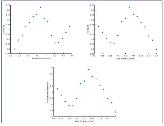
Figure 1: Residual and standard residual plots against independent and dependent variables for the experiment investigating the relationship between wire thickness and sensitivity of electromagnetic probes.
(f) The residuals for the regression model fitted to the data above are summarised in the Table 4, calculate the mean square error of this model.
|
Observation
number
|
Sensitivity
(unitless)
|
Wire thickness
(mm)
|
Fitted values
|
Residuals, e(i)
|
|
1
|
1.51
|
0.05
|
1.5423
|
0.0323
|
|
2
|
1.49
|
0.06
|
1.4593
|
-0.0307
|
|
3
|
1.47
|
0.07
|
1.3763
|
-0.0937
|
|
4
|
1.43
|
0.08
|
1.2934
|
-0.1366
|
|
5
|
1.35
|
0.09
|
1.2104
|
-0.1396
|
|
6
|
1.19
|
0.1
|
1.1274
|
-0.0626
|
|
7
|
0.96
|
0.11
|
1.0445
|
0.0845
|
|
8
|
0.85
|
0.12
|
0.9615
|
0.1115
|
|
9
|
0.65
|
0.13
|
0.8785
|
0.2285
|
|
10
|
0.64
|
0.14
|
0.7955
|
0.1555
|
|
11
|
0.58
|
0.15
|
0.7126
|
0.1326
|
|
12
|
0.56
|
0.16
|
0.6296
|
0.0696
|
|
13
|
0.52
|
0.17
|
0.5466
|
0.0266
|
|
14
|
0.53
|
0.18
|
0.4637
|
-0.0663
|
|
15
|
0.49
|
0.19
|
0.3807
|
-0.1093
|
|
16
|
0.50
|
0.20
|
0.2977
|
-0.2023
|
Table 4: Data from the larger experiment conducted along with predicted values and residuals.