Reference no: EM132571106

EE4108 Machine Learning - Aston University

Problem 1:

Consider a two-dimensional class problem that involves two classes ω₁ (y₁ = 1) and ω₂ (y₂ = 0). Each one of them is modelled by a mixture of equiprobable Gaussian distributions. Specifically, the means of the Gaussians associated with ω₁ are [ 5, 5]^T and [5, 5]^T , while the means of the Gaussians associated with ω₂ are [ 5. 5]^T . [0.0]^T and [5, 5]^T . The covariances of all Gaussians are σ²I where σ² = 2.

i. Using of the mixt model python function that you will be given during one of the lab sessions, generate and plot a data set X1 (training set) containing 100 points from ω1 (50 points from each associated Gaussian) and 150 points from ω2 (again 50 points from each associated Gaussian). In the same way, generate an additional set X₂ (test set). Plot the generated sets in different figures, designating the different points of each class.

ii. Based on X₁, create a two-layer neural network with two nodes in the hidden layer hav- ing the hyperbolic tangent as activation function and a single output node with sigmoid activation function 1. Perform training with the standard back-propagation algorithm for 10000 iterations and step-size equal to 0.5. Compute the calculated costs for every 100 iterations for the training and the test sets, based on X₁ and X2, respectively. Also, make a scatter plot the test points, and plot the decision areas formed by the network in a single figure.

iii. Repeat step (ii) for step-size equal to 0.001 and comment on the results.

iv.Repeat step (ii) for k = 1, 4, 20 hidden layer nodes and comment on the results.

Problem 2:

In this problem we will examine the prediction power of the kernel ridge regression in the presence of noise and outliers. We consider original data were samples are generated from a music recording, such as of the Blade Runner by Vangelis Papathanasiou. Read the audio file using the read function from SoundFile 2 package and take 1000 data samples (starting from the 100,000th sample). Then add white gaussian noise at a 15 dB level and randomly "hit" 50 of the data samples yn with outliers (y_n ± 0.8ymax, i.e. set the outlier induced deviation is 80% of the maximum value of all the data samples).

i. Find the reconstructed data samples using the kernel ridge regression method (see eq. 6.9 of PRML textbook). Employ the Gaussian kernel with σ = 0.004 and set λ = 0.0001.

Plot the fitted curve of the reconstructed samples together with the data used for training.

ii.Repeat the first step (i) using λ = 10^-6, 10^-5, 0.0005, 0.001, 0.01 and 0.05

iii.Repeat the first step (i) using σ = 0.001, 0.003, 0.008 and 0.05

iv.Comment on the above results

Problem 3

In this problem we will examine the performance of a SVM in the context of a two-class two- dimensional classification task. The data set comprises N = 150 points, x_n = [x_n,1, x_n,2]T where n = 1, 2, ..., N , uniformly distributed in [-5, 5] × [-5, 5]. For each point compute:

y_n = 0.05x³_n,1 + 0.05x²_n,1 + 0.05x_n,1 + 0.05 + η

where η denotes zero-mean Gaussian noise of variance σ²_n = 4. Then, if x_n,2 ≥ yn assign it to ω₁, and if x_n,2 < y_n assign it to class ω₂.

i. Plot the points [ x_n,1, x_n,2] using different colors for each class.

ii. Obtain the SVM classifier from Ski-learn or any other related Python package. Use the Gaussian kernel with σ = 20 and set C = 1. Plot the classifier and the margin (for the latter you can employ the contour function from Matplotlib package 3). Moreover, find the support vectors (i.e. the points with nonzero Lagrange multipliers that contribute to the expansion of the classifier) and plot them as circled points.

iii. Repeat the ii-step using C = 0.5, 0.1 and 0.005. Repeat again using C = 5, 10, 50 and 100

iv. Comment on the results

Problem 4

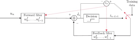
Consider the decision feedback equalizer depicted in the above figure.

i. Generate a sequence of 1000 random ±1 samples, representing a transmitted BPSK signal (i.e. sn). Direct this sequence into a linear channel with impulse response h = [0.04, -0.05, 0.07, -0.21, 0.72, 0.36, 0.21, 0.03, 0.07]^T and add to the output 11dB white Gaussian noise using the given py awgn function. Denote the output as un.

ii. Design the adaptive decision feedback equalizer (DFE) using L = 21, l = 10, and µ = 0.025 following the training mode only. Perform a set of 500 experiments feeding the DFE with different random sequences from the one described in step (i). Plot the mean square error (averaged over the 500 experiments). Observe that around n = 250 the algorithm achieves convergence.

iii. Design the adaptive decision feedback equalizer using the parameters of step-(ii). Feed the equalizer with a series of 10,000 random values generated as in step-(i). After the 250th data sample, change the DFE to decision-directed mode. Count the percentage of the errors performed by the equalizer from the 251th to the 10,000th sample.

iv. Repeat steps (i) and (ii) changing the level of the white Gaussian noise added to the BPSK values to 15, 12, 10 dB. Comment on the results.

Attachment:- Machine Learning.rar