Reference no: EM132153999
SIGNALS & SYSTEMS ASSIGNMENT - Analysing a system
A vehicle suspension system can be modelled by the block diagram shown in Figure 1 below:
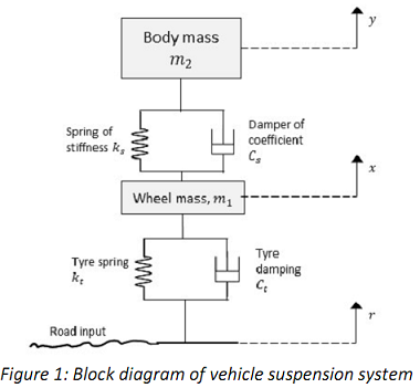
In this block diagram, the variation in the road surface height r as the vehicle moves is the input to the system. The tyre is modelled by the spring and dashpot (damping) system with spring constant kt and damping coefficient Ct respectively and this results in the displacement of the wheel (x), represented by the mass m1. The wheel's displacement acts as an input to the suspension system, modelled by the spring and dashpot with spring constant ks and damping coefficient Cs respectively and this results in the displacement (y), of the body, represented by the mass m2. When the car is at rest, it is taken that r = 0, x = 0 and y = 0. (Note: m2 is normally a quarter of the vehicle mass since it is assumed the weight is distributed evenly between the 4 wheels.
This system is composed of two mass-spring-damper systems 'stacked' one on top of the other. We shall first consider the behaviour of a single sub-system and then later combine these to find the overall system behaviour.
Consider the simple mass-spring damper system shown in Figure 2 below:
In Figure 2:
- x is the position of input body/surface, with its rest position given by x = 0.
- The mass m represents the mass
- The height of mass m above its reference level is called y. The reference level is chosen such that when system is at rest, y = 0.
Section 1: Mathematical Analysis of System
1. Draw a free-body diagram showing all the forces acting on the mass m shown in Figure 2.
2. From the earlier description, diagrams and the laws of Physics, show that the motion of the system in Figure 2 can be described by the LCCDE (linear constant-coefficient differential equation) below:
d2y(t)/dt2 + C/m dy(t)/dt + k/m y(t) = C/m dx(t)/dt + k/m x(t) (1)
3. Using the Laplace transform of the equation above, find an expression for H(s), the system transfer function.
The mass-spring-damper system is a damped second order system. It is common to express the homogenous second order DE for such a damped system as
d2y(t)/dt2 + 2ζωn dy(t)/dt + ω2ny(t) = 0 (2)
where ζ is the damping ratio and ωn is the undamped natural (resonant) frequency.
4. From equations (1) and (2), determine expressions for ζ (the damping ratio) and ωn (the natural frequency) in terms of the parameters m, k and C.
5. Determine the characteristic equation and eigenvalues (characteristic values) for this system based on equation (2) above.
6. From the answer to part 5, determine the natural response of the system for the following cases:
a. ζ = 0
b. 0 < ζ < 1
c. ζ = 1
d. ζ > 1
Consider a suspension system with the following parameters:
m2 = 340 kg
ks = 21,000 N/m
7. Determine ωn (in rad/s) for this suspension system and the corresponding value for fn (in Hz).
8. Calculate the required value of Cs in order to achieve ζ = 1.
Note: Complete and clear working is required for all answers for this section.
Section 2: System analysis using Matlab
In this section, the system responses should be analysed using Matlab. Refer to the document "A Brief MATLAB Guide" in order to understand how to represent LTI systems in Matlab, and hence how to determine impulse response, step response and frequency response of systems. Students are advised to refer to the help function within Matlab as well as online Matlab documentation for more details.
MATLAB is installed in the engineering computer labs.
Using the commands given in the Guide, analyse the response of the suspension system using the m2 and ks parameters given in Section 1 and Cs value calculated in question 8:
9. Plot the impulse response and step response of the system (for 2 seconds duration and time 'step size' of 1 millisecond) using the impulse and step functions. Include all plots (properly labelled) in your submission.
10. Determine the frequency response from 0 to 200 rad/s using the freqs command. Plot the magnitude and phase response over this frequency range. Hint: Use frequency 'step size' of 0.1 rad/s.
Hint 1: You can plot all 4 graphs in one go using a 2 x 2 matrix of plots using subplot(22n), where n determines which of the 4 subplots gets used.
Hint 2: In order to clearly see variations over a range of frequencies, it is best to use a log scale for the frequency and magnitude (phase would still be displayed using linear scale).
The functions loglog (for magnitude) and semilogx (for phase) can be used instead of plot.
11. Determine the magnitude response at ωn. Determine the frequency of the -3dB point (where magnitude = 1 1/√2). Hint: Use the 'data cursor' tool on the plot of the magnitude response. It shows the x and y values of the plot as you move along the curve.
12. Discuss the response of the system. Why do the impulse and step responses have that particular shape? How well will this system fulfil its purpose of a vehicle suspension?
Note: The function of a suspension system is to 'filter out' the effect of bumps, potholes and other such vibrations, but allow the vehicle to 'follow the road' as the height of the road surface varies.
13. Repeat the analysis above (steps 9 - 11) for the following damping ratios
a. ζ = 0.5
b. ζ = 0.7
c. ζ = 1.5
Hint 3: It would be more efficient to put all the necessary commands into a script file (a .m file) so you can edit the parameters and then run all the commands at once.
14. Based on the results of the Matlab analysis above, which of the 4 values of damping ratio would be best for application as a suspension system. Justify your selection.
Section 3: State Space Analysis
A brief introduction to state space analysis
State space analysis enables a system that would be described using an nth order differential equation to be represented using first order matrix differential equations through the definition of n state variables.
The state space representation of a system is given by two equations:
a) The state equation: q· = Aq + Bx
b) The output equation: y = Cq + Dx
Note: The variables in the equation above are denoted in bold as they are matrices.
For an nth order system with r inputs and m outputs, the sizes of the matrices are as below:
|
Matrix
|
Size
|
Name
|
Type
|
|
q
|
n x 1
|
State vector
|
Function of time
|
|
A
|
n x n
|
State matrix
|
Constant
|
|
B
|
n x r
|
Input matrix
|
Constant
|
|
X
|
r x 1
|
Input
|
Function of time
|
|
Y
|
m x 1
|
Output
|
Function of time
|
|
C
|
m x n
|
Output matrix
|
Constant
|
|
D
|
m x r
|
Direct transition (or feedforward) matrix
|
Constant
|
15. Research and discuss the advantages of state space analysis and the types of problems for which state space analysis is most suited (in no more than 500 words).
16. From your research, give one example system described using state space analysis, including all the matrices.
Note: You will need to properly reference your sources (both in-text and end-text).
17. Discuss the approach to and advantages of using state space techniques to analyse the complete suspension system including both tyre and wheel base, as shown in Figure 1.
Note: All referencing must conform to the APA referencing standard (as per ECU referencing standards).
Attachment:- Assignment Files.rar