Reference no: EM132372195
Analysis of Biological Communities
ASSIGNMENT #1: DIVERSITY AND CLUSTER ANALYSIS
BOVID DATA SET
A complete description of these data, and numerous analyses using R, is given in Part 2 of the "R" Manual (Data Set #2, pages 6--19); read over this material carefully, and undertake the exercises and analyses in R on your own. Information required to answer the questions in the Assignment is also presented below.
Here are the data used in all of the analyses.
|
PARK
|
ant
|
alc
|
hip
|
red
|
tra
|
neo
|
cep
|
aep
|
bov
|
|
NGO
|
13.889
|
37.861
|
0
|
0.333
|
1.111
|
0
|
0
|
0
|
0.167
|
|
TUR
|
0.517
|
0.987
|
0.655
|
0
|
0
|
0
|
0
|
0
|
0
|
|
ETO
|
0.539
|
0.207
|
0.215
|
0
|
0.112
|
0.022
|
0.011
|
0
|
0
|
|
KAL
|
0.655
|
0.56
|
0.438
|
0
|
0.179
|
0.045
|
0.019
|
0
|
0
|
|
SER
|
7.451
|
17.843
|
0.196
|
0.216
|
0.373
|
0
|
0
|
2.549
|
1.961
|
|
NAI
|
6.926
|
11.049
|
0
|
0.861
|
0.639
|
0.016
|
0.016
|
5.189
|
0
|
|
KAF
|
0
|
2.088
|
0.341
|
2.176
|
0.462
|
0.989
|
0.33
|
0.022
|
0.934
|
|
BIC
|
0
|
0.063
|
0.063
|
0.019
|
0.057
|
0.019
|
0.063
|
0.019
|
0.013
|
|
LUA
|
0
|
0
|
0.362
|
0.272
|
0.109
|
0.03
|
0.133
|
0
|
0.018
|
|
CUE
|
0
|
0.056
|
0.044
|
0.356
|
0.167
|
0.222
|
0.111
|
0
|
0
|
|
HLU
|
0
|
3.655
|
0
|
1.051
|
3.335
|
0
|
0.016
|
5.098
|
2.286
|
|
MKU
|
0
|
4.325
|
0
|
0.214
|
1.65
|
0.019
|
0.012
|
29.084
|
0
|
|
WAN
|
0
|
0.198
|
0.197
|
0.094
|
0.41
|
0.226
|
0.15
|
0.602
|
0.977
|
|
QUI
|
0
|
0
|
0.151
|
0.151
|
0.552
|
0
|
0.351
|
0
|
0.803
|
|
KRU
|
0
|
0.524
|
0.073
|
0.248
|
0.583
|
0.267
|
0.068
|
8.017
|
1.268
|
|
MAN
|
0
|
0
|
0
|
0.591
|
0.269
|
0
|
0
|
7.527
|
16.129
|
TABLE 1. Raw data file: abundance values (as number of animals per km2) for 9 herbivore tribe groups (variables, data columns) in 16 African game parks (individuals, data rows).
Refer to information and analyses on pages 6--12 of the "R" Manual Part 2 (Data Set #2)
Question 1:
[Richness, effective richness and evenness values are given in TABLE 2; from page 11 of "R" Manual]
(a) Summarize and discuss trends in the herbivore tribe group richness (N0 = S) across the 16 parks (e.g. which parks have the highest and lowest number of tribe; what is the range of values; and so forth).
(b) Summarize and discuss trends in the effective richness N1 (Shannon Index) and N2 (Simpson Index) of herbivore tribe groups across the 16 parks (e.g. highest and lowest values, range of values, and so forth). Do high values of richness (N0 = S) always correspond high values for N1 and N2); if not, why not? HINT: e.g. compare parks with high N0 = 8; why do the N1 and N2 values differ among these 3 parks? Provide examples to support your answer [refer to raw data, TABLE 1].
(c) Summarize the evenness (E21) values across the 16 parks. Why do parks KRU and MKU have relatively low evenness? Why does park TUR have the highest evenness value, even though it has the lowest herbivore tribe group richness (N0 = 3)? Use the raw data values (TABLE 1) to support your answer.
EFFECTIVE RICHNESS ALPHA-VALUE EVENNESS
|
PARK
|
0
|
0.25
|
0.5
|
1
|
2
|
4
|
8
|
16
|
32
|
64
|
Inf
|
E12 = (N2-1)/(N1-1)
|
|
NGO
|
5
|
3.447
|
2.663
|
2.063
|
1.749
|
1.571
|
1.48
|
1.442
|
1.425
|
1.417
|
1.409
|
0.705
|
|
TUR
|
3
|
2.973
|
2.946
|
2.892
|
2.79
|
2.623
|
2.431
|
2.304
|
2.243
|
2.215
|
2.187
|
0.946
|
|
ETO
|
6
|
5.138
|
4.539
|
3.811
|
3.115
|
2.566
|
2.273
|
2.153
|
2.1
|
2.075
|
2.052
|
0.752
|
|
KAL
|
6
|
5.234
|
4.723
|
4.152
|
3.71
|
3.43
|
3.236
|
3.091
|
2.995
|
2.944
|
2.895
|
0.860
|
|
SER
|
7
|
5.359
|
4.3
|
3.199
|
2.434
|
2.031
|
1.851
|
1.777
|
1.744
|
1.729
|
1.714
|
0.652
|
|
NAI
|
7
|
5.062
|
4.224
|
3.544
|
3.078
|
2.748
|
2.498
|
2.358
|
2.294
|
2.264
|
2.235
|
0.817
|
|
KAF
|
8
|
7.059
|
6.424
|
5.606
|
4.735
|
4.066
|
3.714
|
3.559
|
3.482
|
3.436
|
3.374
|
0.811
|
|
BIC
|
8
|
7.633
|
7.304
|
6.765
|
6.086
|
5.553
|
5.291
|
5.168
|
5.098
|
5.057
|
5.016
|
0.882
|
|
LUA
|
6
|
5.37
|
4.889
|
4.247
|
3.62
|
3.16
|
2.878
|
2.715
|
2.631
|
2.591
|
2.552
|
0.807
|
|
CUE
|
6
|
5.642
|
5.324
|
4.805
|
4.13
|
3.503
|
3.081
|
2.868
|
2.772
|
2.728
|
2.685
|
0.823
|
|
HLU
|
6
|
5.209
|
4.856
|
4.53
|
4.198
|
3.837
|
3.498
|
3.26
|
3.139
|
3.083
|
3.029
|
0.906
|
|
MKU
|
6
|
3.532
|
2.539
|
1.818
|
1.437
|
1.295
|
1.248
|
1.23
|
1.221
|
1.218
|
1.214
|
0.534
|
|
WAN
|
8
|
7.472
|
6.978
|
6.121
|
4.95
|
3.949
|
3.394
|
3.138
|
3.024
|
2.971
|
2.921
|
0.771
|
|
QUI
|
5
|
4.742
|
4.508
|
4.119
|
3.605
|
3.141
|
2.83
|
2.658
|
2.576
|
2.537
|
2.501
|
0.835
|
|
KRU
|
8
|
5.925
|
4.423
|
2.775
|
1.832
|
1.533
|
1.443
|
1.408
|
1.392
|
1.385
|
1.378
|
0.469
|
|
MAN
|
4
|
3.147
|
2.641
|
2.176
|
1.895
|
1.721
|
1.613
|
1.563
|
1.541
|
1.53
|
1.52
|
0.761
|
TABLE 2. Richness (N0) and effective richness Nα [for various α--values (columns)] of tribal groups for each of the 16 African game parks. Evenness values E12 are given at the far right.
Refer to the "R" manual (Data Set #2, pages 6--12) for information on obtaining these values using "R".
Question 2.
(a) To what degree are the diversity measures N0 N1, N2 and E21 correlated for these data? Refer to the correlation matrix (TABLE 3), and the pairwise scatterplots (FIGURE 1).
(b) Discuss why these measures are, or are not, correlated, e.g. why are N1 and N2 highly correlated, but not N0 and N1?; why is E12 poorly correlated with Nα?; and so forth.
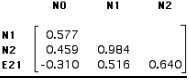
TABLE 3. Pairwise correlation matrix of diversity (N0, N1, N2) and evenness (E21) values.
FIGURE 1. All six pairwise scatterplots for the diversity (N0, N1 and N2) and evenness (E21) values.
Question 3:
(a) Examine, and briefly summarize, the Renyi diversity profiles (as effective richness Nα) for the 16 parks (FIGURE 2).
(b) Compare the results for parks KRU, MAN, BIC and TUR, relating the differences in these four profiles to their corresponding bovid tribe abundance distributions (given in TABLE 1).
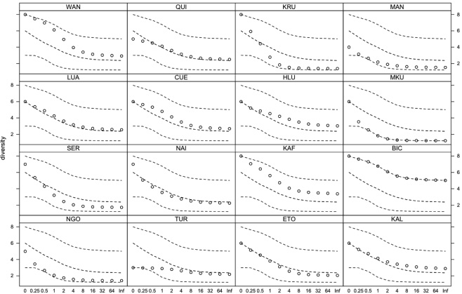
FIGURE 2. Renyi Diversity (as effective richness, Nα) Profiles for the 16 African game parks [α--values on horizontal axis, effective richness Nα on vertical axis]. NOTE: α = 0, species richness; α = 1, Shannon index; α = 2, Simpson Index; α = Inf (infinity), Berger--Parker index. Observed values are shown as open circles. The upper and lower dashed lines are the upper (maximum) and lower (minimum) bounds for the data, across all 16 parks. The middle dashed line represents the mean values, averaged across all 16 parks.
CLUSTER ANALYSIS: BOVID TRIBES IN AFRICA
The R commands to produce these results are given in Part 2 of the "R" Manual, pages 13--15.
Note that for all of the cluster analyses undertaken, CHORD DISTANCE was utilized.
Question 4:
(a) Why was Chord Distance, rather than Euclidean distance, used to quantify the associations among the 16 African game parks?
(b) What aspect of the data would have been emphasized if Euclidean Distance had been used? Summarize how the standardization "built into" Chord Distance alleviates this problem.
Question 5:
(a) Compare the dendrograms of Single and Complete Linkage cluster analyses of the 16 parks (FIGURE 3). How similar are the two dendrograms, and how do they differ?
(b) What do the similarities/differences between the Single and Complete Linkage dendrograms tell you about the robustness of group structure in the bovid tribe data?
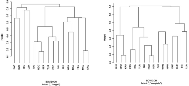
FIGURE 3. Cluster analysis dendrograms of 16 parks (based on Chord Distance), using single linkage or nearest neighbour (left) and complete linkage or furthest neighbour (right).
Question 6:
(a) Compare and contract group structure of Single, Complete, Average, and Ward (Sum of Squares) dendrograms for the 16 parks, at the 4--group level (FIGURE 4).
(b) Which cluster methods produce similar/different 4--group results? Summarize your findings in tabular format.
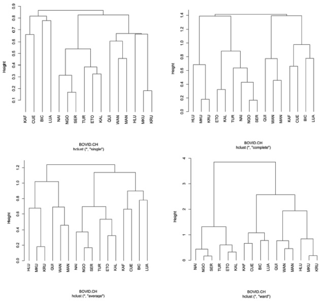
FIGURE 4. Cluster analysis dendrograms of 16 parks (based on Chord Distance), using single linkage or nearest neighbour (top left), complete linkage or furthest neighbour (top right), average linkage or UPGMA (bottom left), and Ward's or sum of squares (bottom right).
Question 7:
HINT: in answering this question, refer to and interpret the sorted Bovid Density file (with data standardized to percent abundance, i.e. sum of values for each park = 100%) shown in TABLE 4.
(a) Using the sums of squares cluster dendrograms for the 16 parks, and for the 9 tribes (FIGURE 5), summarize (in tabular format) and comment on the relationships between the bovid parks at the 4--group level and the 9 tribes at the 3--group level.
(b) Which tribe groups are most affiliated with which park groups?
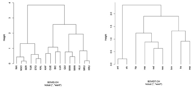
FIGURE 5. Sum of squares cluster analysis dendrograms of the 16 parks based on Chord Distance (left), and of the 9 tribes based on Chord Distance (right).
|
|
Tribe gp. ->
|
1
|
1
|
2
|
2
|
2
|
2
|
3
|
3
|
3
|
|
Park Gp.
|
PARK
|
ant
|
alc
|
hip
|
cep
|
red
|
neo
|
bov
|
tra
|
aep
|
|
1
|
NAI
|
28.0
|
44.7
|
0.0
|
0.1
|
3.5
|
0.1
|
0.0
|
2.6
|
21.0
|
|
1
|
NGO
|
26.0
|
71.0
|
0.0
|
0.0
|
0.6
|
0.0
|
0.3
|
2.1
|
0.0
|
|
1
|
SER
|
24.4
|
58.3
|
0.6
|
0.0
|
0.7
|
0.0
|
6.4
|
1.2
|
8.3
|
|
1
|
TUR
|
23.9
|
45.7
|
30.3
|
0.0
|
0.0
|
0.0
|
0.0
|
0.0
|
0.0
|
|
1
|
ETO
|
48.7
|
18.7
|
19.4
|
1.0
|
0.0
|
2.0
|
0.0
|
10.1
|
0.0
|
|
1
|
KAL
|
34.5
|
29.5
|
23.1
|
1.0
|
0.0
|
2.4
|
0.0
|
9.4
|
0.0
|
|
2
|
KAF
|
0.0
|
28.4
|
4.6
|
4.5
|
29.6
|
13.5
|
12.7
|
6.3
|
0.3
|
|
2
|
CUE
|
0.0
|
5.9
|
4.6
|
11.6
|
37.2
|
23.2
|
0.0
|
17.5
|
0.0
|
|
2
|
BIC
|
0.0
|
19.9
|
19.9
|
19.9
|
6.0
|
6.0
|
4.1
|
18.0
|
6.0
|
|
2
|
LUA
|
0.0
|
0.0
|
39.2
|
14.4
|
29.4
|
3.2
|
1.9
|
11.8
|
0.0
|
|
3
|
QUI
|
0.0
|
0.0
|
7.5
|
17.5
|
7.5
|
0.0
|
40.0
|
27.5
|
0.0
|
|
3
|
WAN
|
0.0
|
6.9
|
6.9
|
5.3
|
3.3
|
7.9
|
34.2
|
14.4
|
21.1
|
|
3
|
MAN
|
0.0
|
0.0
|
0.0
|
0.0
|
2.4
|
0.0
|
65.8
|
1.1
|
30.7
|
|
4
|
HLU
|
0.0
|
23.7
|
0.0
|
0.1
|
6.8
|
0.0
|
14.8
|
21.6
|
33.0
|
|
4
|
MKU
|
0.0
|
12.3
|
0.0
|
0.0
|
0.6
|
0.1
|
0.0
|
4.7
|
82.4
|
|
4
|
KRU
|
0.0
|
4.7
|
0.7
|
0.6
|
2.2
|
2.4
|
11.5
|
5.3
|
72.6
|
TABLE 4. Sorted and standardized Bovid Data Set (data from Table 1). The rows and columns are sorted according to cluster group affinities (4 groups for parks, 3 groups for tribes, see Figure 5). In addition, the tribal abundances are expressed as a percentage within each park (i.e. values for a given park sum to 100%).