Reference no: EM13983

Q1 Filter function form is y = myfilter(x,b,a) where x is input, y is output and a and b are the IIR and FIR coefficients.

In the transfer function, the matrix "a" indicates the denominator coefficients and the matrix "b" is numerator coefficients.

I use command "global buffer;" to set a global variable as the shift buffer.

For a second order IIR filter, the transfer function is like:

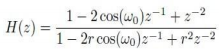
Where w0 is stopband filter frequency, r is the stopband width.

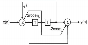
The signal flow diagram is:

From the diagram, I work out the function in Matlab:
output=b(2)*buffer(1);
input=input-a(2)*buffer(1);
output=output+b(3)*buffer(2);
input=input-a(3)*buffer(2);
output=output+input*b(1);

When the output is figured out, the input is set to buffer(1) and the buffer(1) becomes buffer(2).
buffer(2)=buffer(1);
buffer(1)=input;

Q2

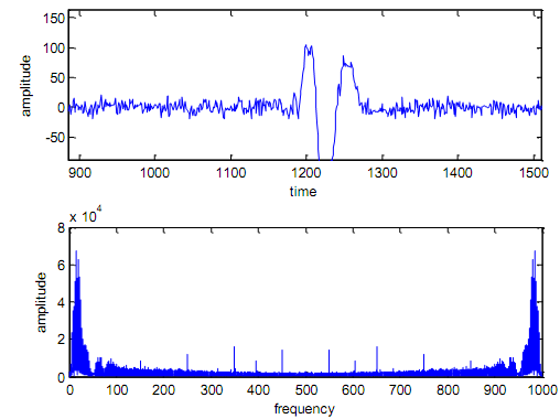
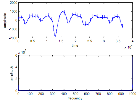
I use the command "load ('1104111.txt')" to load my ecg file. The signal minus 2048 to make it range from -2048mV to +2048mV.

And plot the original signal.

To eliminate the 50Hz hum, so I make w0=2*pi*50/fs; r refers to the width of the stopband. And the closer r goes to 1, the more narrow is the stopband. I choose r=0.93.

Because it is a second order filter so the buffer contains 2 components.

To define the buffer in advance, I use the command of "global buffer;buffer=zeros(2,1);"

The coefficients a and b are:
b1=1; b2=-2*cos(w0); b3=1;
a1=1; a2=-2*r*cos(w0); a3=r^2;
b=[b1,b2,b3]; a=[a1,a2,a3];

Then a loop is used for filtering the whole signal.
op1=zeros(l,1);
for k=1:l
op1(k)=myfilter_3(ecg1(k),b,a);
end

Plot the result.

Q3

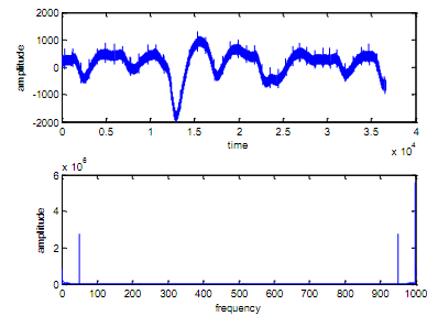
In this section, the steps are similar with the Q2.
To eliminate the DC component, w0=0;
The other steps are almost same as the Q2.
The result is plotted as:

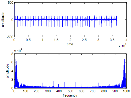
At last, to check the PQRST peaks, zoom in the plot