Reference no: EM132154390

Mathematical Economics Assignment Questions -

Q1. Find the equilibrium solution for each of the following models.

(a) Q_d = Q_s, Q_d = 210 - 2P², Q_s = 8P + 120

(b) Q_d = Q_s, Q_d = 496 - 0.25P², Q_s = 2P² - 80

Q2. Determine P_i* and Q_i* (I = 1, 2) for the demand and supply functions of the two-commodity market given below. Express your answer using fractions rather than decimals.

Q_d1 = 27 - 3P₁ + P₂, Q_d2 = 18 + 2P₁ - 3P₂, Q_s1 = -4 + 4P₁ - 3P₂, Q_s2 = -2 - 3P₁ +5P₂

Q3. A society has three states of wealth: rich, middle income and poor. The initial, time t = 0, proportions of the population in each state are rich R₀ = 0.2, middle income M₀ = 0.7 and poor P₀ = 0.1. Let v^→_n = (R_n M_n P_n) denote the vector of proportions after n time periods. The transition from one state to another over a single time period is determined by

R_n+1 = 0.8R_n +0.1M_n

M_n+1 = 0.1R_n +0.4M_n +0.2P_n

P_n+1 = 0.1R_n +0.5M_n +0.8P_n

(a) Determine the transition matrix T so that v^→_n+1 = (R_n+1 M_n+1 P_n+1) = v^→_nT.

(b) Determine the portions of the population in each state after one and two time periods.

(c) Let v^→_S^T = (R_S M_S P_S) denote the vector of steady state proportions. Thus,

v^→_ST = v^→_S ⇒ T^Tv^→_S^T = v^→_S^T,

and hence v^→_S^T is a solution to system

(I -T^T)x^→ = 0^→. (1)

Determine v^→_S by first using Gauss-Jordan elimination to solve Equation 1 and thereby determine v^→_S^T.

Q4. Suppose the technology of the economy is given by the following input/output matrix A, and labor/output vector l^→,

as the consumption vector.

Using this information, the augmented input coefficients matrix can be calculated as B = A +c^→l^→. The characteristic polynomial of B is given by, p(λ) = λ³ - 0.6λ² - 0.25λ - 0.018.

The matrix B has three distinct real eigenvalues λ₁, λ₂, and λ₃ with corresponding eigenvectors,

(a) Determine B.

(b) Use the eigenvectors given above to estimate the value of any positive eigenvalues of B. Hint: Compute the first (or second or third) component of Bv^→_i and check to see if it is a positive multiple of the first (or second or third) component of v^→_i.

(c) Determine the technically maximum feasible growth rate for this economy.

Q5. Given

	Agriculture	Manufacturing	Services	Other	Final Demand	Total Output
Agriculture	30	70	50	50	50	$250
Manufacturing	80	50	80	70	70	$350
Services	50	30	60	65	45	$250
Other	60	75	30	40	45	$250
Value added	30	125	30	25
Total Input	250	350	250	250
Table 1 - Interindustry Transaction Matrix (Values)

Use Table 1 and the given Leontief inverse to answer the following.

(a) Determine the Technology Matrix.

(b) Determine the increase in the size of the economy caused by a $1 increase in the final demand for services.

(c) Determine the total outputs vector x^→₁ if final demands changes from.

(d) Observe that ∂x_i/∂d_j denote the partial derivative of the total output from sector i with respect to final demand from sector j and that

∂x^→/∂d_j = (∂x₁/∂d_j ∂x₂/∂d_j ∂x₃/∂d_j ∂x₄/∂d_j)^T

denotes the vector of partial derivatives from each sector with respect to final demand from sector j.

Determine ∂x₂/∂d₃ and ∂x^→/∂d₄.

Q6. Given the input matrix and the final demand vector

(a) Write out the specific input-output matrix equation for this model.

(b) Check whether the data in this problem satisfy the Hawkins-Simon condition.

(c) Use Gauss-Jordan elimination or Cramer's Rule to solve the specific equation. You could complete the following Gauss-Jordan elimination calculation,

Q7. Consider an economy with three goods, q^→ = (q₁ q₂ q₃). Let Y denote the income. Suppose the demand and supply functions for these goods are as follows:

Demand	Supply
q1d = -2p1 + p2 -2p3 +0.05Y	q1s = 4p1 - 3p2 + p3 -15
q2d = p1 -2p2 + p3 +0.1Y	q2s = -3p1 +4p2 - p3 - 30
q3d = -2p1 + p2 - 4p3 +0.04Y	q3s = p1 - p2 +2p3 - 12

(a) Interpret the signs of the coefficients of price and income variables in the demand functions?

Hint: Why should the demand for a good be affected by a change in the price of another good? Notice the symmetric nature of the signs of coefficients.

(b) Suppose Y = 900. Find the equilibrium prices for this three good economy.

(c) What happens to the prices when income (Y) increases to 1,350.

Q8. Given the average-cost function AC = 1/5Q² - 1.2Q + 50 + 42/Q, find the MC function. Is the given function more appropriate as a long-run or short-run function? Why?

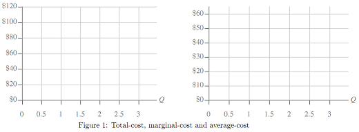
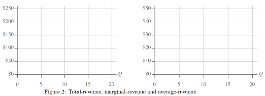
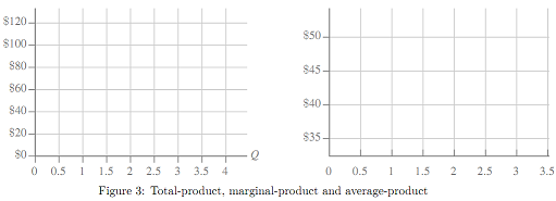
Q9. Find the marginal and average functions for the following total functions and graph the results.

(a) Total-cost function: TC = 8Q² +4Q+24

(b) Total-revenue function: TR = -2.5Q² + 50Q

(c) Total-product function: TP = -5L³ +25L² + 10L

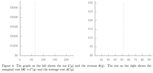
Q10. Let C = 0.004(q-20)³ + 8(q-20) + 692 be the total cost function, and let p(q) = 64 - 0.25q be the price function so that revenue is given by R(q) = qp(q) = 64q - 0.25q².

(a) Add to the left panel of Figure 4 the graphs of C(q) and R(q) on the same set of axes. You will need to use calculus to determine the concavity, any inflection points and any local maxima or minima.

(b) Determine a formula for the profit π(q). By solving the first order condition and checking the second order, show that profit is maximized at q* = 64.49. Add to your diagram from part 10a lines tangent to the graphs of C(q) and R(q) at (q*, C(q*)) and (q*, R(q*)). Comment on the relationship between these two lines. Hint: Use R(q) = -0.25(q-20)² +54(q-20) +1180, also, (0.5±√((-0.5)²-4(-0.012)(46)))/2(-0.012) = -20.83±65.33 = -86.16 or 44.49.

(c) Add to the right panel of Figure 4 the graphs of the marginal cost MC = C'(q) and the average cost AC = C(q)/q on the same set of axes. You will need to use calculus to determine the concavity, any inflection points and any local maxima or minima. Comment on the quantity q** at which the two graphs intersect. Hint: q** ≈ 52.59 as MC(q**)-AC(q**) = 0.0000010660.

Q11. The total money supply M has two components: bank deposits D and cash holdings C, which we assume to bear a constant ratio C/D = c, 0 < c < 1. The high-powered money H is defined as the sum of cash holdings held by the public and reserves held by the banks. Bank reserves are a fraction of bank deposits, determined by the reserve ratio r, 0 < r < 1.

(a) Express the money supply M as a function of the high-powered money H.

(b) Would an increase in the reserve ratio r raise or lower the money supply?

(c) How would an increase in the cash-deposit ratio c affect the money supply?

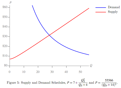
Q12. Given the supply and demand schedules P = 7 + Q²_S/(Q_S+4) and P = 55566/(Q_D +14)².

(a) Confirm that the equilibrium price and supply are given by P* = $31.5 and Q* = 28.

(b) Give formulas for dP/dQ_S and dP/dQ_D and their numerical values at Q* = 28.

dP/dQ_S = d/dQ_S[7 + Q²_S/(Q_S+4)] =

dP/dQ_D = d/dQ_D[55566/(Q_D+14)²] =

(c) Determine the equilibrium price elasticities of demand, ε_{Q_D/P} and supply, ε_{Q_S/P}.

ε_{Q_D/P} = dQ_D/dP P/Q_D = 1/(dP/dQ_D) P/Q_D =

ε_{Q_S/P} = dQ_S/dP P/Q_S = 1/(dP/dQ_S) P/Q_S =

(d) Determine the linear (tangent line) approximations to the supply and demand schedules at P* = $31.5 and Q* = 28. Add graphs of these lines to Figure 5.

Supply: P ≈ P* + dP/dQ_S|_{Q_S=Q*} (Q_S - Q*) =

Demand: P ≈ P* + dP/dQ_D|_{Q_D=Q*} (Q_D - Q*) =

Q13. The supply function of a certain commodity is Q = a(R - bR²)P^c [R: rainfall]

Find the price elasticity of supply ε_Q/P and the rainfall elasticity of supply ε_Q/R.

Q14. The foreign demand for our exports X depends on the foreign income Y_f and our price level P: X = aY_fe^-bP. Find the partial elasticity of foreign demand for our exports with respect to our price level, ε_X/P, and the partial elasticity of foreign demand for our exports with respect to the foreign income, ε_X/Y_f.

Q15. Find the rate of change of output with respect to time, if the production function is Q = A(t)K^αL^β, where A(t) is an increasing function of t and K = K₀ +at and L = L₀ +bt.

Q16. (a) A wine dealer is in possession of several cases of wine which he can either sell at the present time (t = 0) for $K or else store for some length of time and then sell at a higher value. The growing value (V) of the wine is given by V = 2K/(1+e^-rt). Assuming a discount rate of r (on a continuous basis), how long should the dealer plan to store the wine in order to maximize its present value?

Q17. Suppose the demand for money M_d is a function of national income Y = Y(t) and the interest rate i = i(t). Let ε_{M_d} /Y and ε_{M_d}/I denote the elasticities of M_d with respect to Y and i. Show that the rate of growth of M_d can be expressed as the weighted sum of the rates of growth of Y and i, r_Y and r_i,

r_{M_d} = ε_{M_d/Y} r_Y +ε_{M_d/I} r_i.

Q18. Given the production function Q = F(K,L), find the general expression for the rate of growth of Q in terms of the rates of growth of K and L.

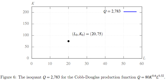
Q19. Suppose that production is given by the Cobb-Douglas production function Q = 80K^0.6L^0.32.

(a) Show that Q is homogeneous and determine the degree of homogeneity k.

(b) What type of returns to scale does production show?

(c) Verify that Euler's theorem for homogeneous functions holds.

(d) Add to Figure 6 the graph of the isoquant which passes through the point (L₀, K₀) = (20, 75). You could try using gnuplot,

Q(K, L)= 80*K** 0.6*L** 0.32 ; Iso(Q, L) = (Q/(80*L** 0.32))** 1.66667

Qfixed= Q(75, 20)

plot [L=0:3*20] [K=0:3*75] Iso(Qfixed,L)

(e) Determine a simple formula for the marginal rate of technical substitution, MRTS.

(f) Determine the slope m of the isoquant at (L₀, K₀) = (20, 75).

(g) Give an economic interpretation of MRTS at (L₀, K₀) = (20, 75).

Q20. The equations defining a model of two trading nations are given by

Y₁ = C₁ + I₁* + X₁ - M₁, Y₂ = C₂ + I₂* + X₂ - M₂

C₁ = 0.625Y₁ + 120, C₂ = 0.75Y₂ + 400

M₁ = 0.3Y₁, M₂ = 0.4Y₂

If I₂* = 100, find the value of I₁* if the balance of payments is -100. Hint: construct a system of three equations for the three unknowns Y₁, Y₂ and I₁*.

Q21. The demand functions for a firm's domestic and foreign markets are P₁ = 111 - 13Q₁ and P₂ = 71 - 4Q₂. The firm's total cost function is TC = 23 + 7Q, where Q = Q₁ + Q₂.

(a) Give a formula for the firm's profit function π. Hint: π = TR₁ +TR₂ -TC = P₁Q₁ +P₂Q₂ -TC.

(b) Assume the firm is able to engage in price discrimination. Write down and solve the FONC for a pair of outputs Q₁* and Q₂* to give a profit maximum. Determine the corresponding prices P₁* and P₂* as well as the maximum profit π*.

(c) Check the 2^nd order conditions by first writing down the Hessian, H, and then checking the signs of detH and ∂²π/∂Q₁².

Q22. A monopolistic firm produces two substitute goods x and y. The prices of the two goods p_x and p_y and the cost C of production are related to the quantities produced by the equations,

p_x = 108 - 4x - 2y, p_y = 144 - 2x - 6y and C = 3x² + 6xy + 4y². (2)

(a) Show that the profit maximizing level of outputs are given by x¯ = 4 and y¯ = 5.2.

Determine the maximum profit π¯ and the prices p¯_x and p¯_y.

(b) Check the second order condition to show that the values given indeed give a maximum.

Q23. The constant elasticity of substitution, CES, production function

Q = 4(0.75K^-2.5 + (1-0.75)L^-2.5)^-1/2.5, (3)

determines a firm's output. Suppose production costs are limited to $1,200, the wage rate is $3 per unit of labor, and the rental rate for capital is $9 per unit of capital. Complete the steps below determine the amounts of labor and capital, K* and L*, that give the maximum output Q* subject to the budget constraint. The method of Lagrange multipliers will be used.

(a) Write down the Lagrangian for this problem.

(b) Show that the firm's maginal products of capital and labor are given by,

MP_K = ∂Q/∂K = 0.0234 [Q/K]^3.5 and MP_L = ∂Q/∂L = 0.00781[Q/L]^3.5 (4)

(c) Write down the first order necessary conditions for this problem.

(d) Solve the first order necessary conditions for this problem to show that K* = 100, L* = 100, λ* = 0.3333 and Q* = 400.

(e) Given ∂²Q/∂K²(K*, L*) = -0.02625, ∂²Q/∂L∂K (K*, L*) = 0.02625 and ∂²Q/∂L² (K*, L*) = -0.02625, write down the bordered Hessian H¯ at (K, L) = (K*, L*). Use the bordered Hessian H¯ to test the second order conditions and show that the values determined do yield a maximum.

(f) Interpret the λ you obtained.

(g) Use the envelope theorem to estimate the change in the optimal value of Q if wages rise by 0.25 from 3 to 3.25.

Q24. An electric company is setting up a power plant and must plan its capacity. Demand is given by,

P₁ = 960 - Q₁ Peak-Period Demand

P₂ = 900 - Q₂ Off Peak Demand.

The variable cost is v = 15 per unit (paid in both markets) and capacity costs k = 32 per unit and is paid once but used in both periods.

(a) Write out the Lagrangian and Kuhn-Tucker conditions for this problem.

(b) Carefully check the Kuhn-Tucker conditions and find the optimal outputs and capacity for this problem.

(c) How much of the capacity is paid for by each market?

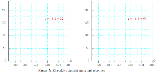
(d) Illustrate the case k = 32 by adding appropriate graphs and labels to the left panel of Figure 7.

(e) Now suppose the capacity costs are k = 90 per unit. Find the quantities, capacity, and how much of the capacity is paid for by each market.

(f) Illustrate the case k = 90 by adding appropriate graphs and labels to the right panel of Figure 7.

Q25. A consumer's diet consists entirely of doughnuts and salads. The consumer can spend up to $15 but must consume no more than 12,000 kilojoules. Doughnuts cost $0.75 each and contain 1,500 kilojoules while salads cost $3 each and contain 400 kilojoules.

Let x and y denote respectively the quantity of doughnuts and salads consumed. The consumer's utility is given by,

u = xy. (5)

Complete the following steps to determine the consumption bundle x*, y* which maximizes the consumer's utility using the method of concave programming.

For convenience let p_x, p_y, k_x, k_y, B and K denote the prices and kilojoule contents (measured in 100's), the budgetary and dietary constraint values. (p_x = 0.75, p_y = 3, k_x = 15, k_y = 4, B = 15, K = 120.)

(a) Determine equations for the objective function and the two constraints.

(b) Determine the (quasi-)concavity or (quasi-)convexity of the objective and constraints.

(c) Write out the Lagrangian and Kuhn-Tucker conditions for this problem.

Since utility is zero if either x = 0 or y = 0 and positive values of utility are possible, it follows that

x* > 0 and y* > 0. (6)

There are four remaining possibilities which may satisfy the Kuhn-Tucker conditions. These correspond to none, one or both of the constraints being binding.

(d) Show that the assumption that both constraints are non-binding leads to a contradiction of the Kuhn-Tucker conditions.

(e) Show that the assumption that the budget constraint is binding but the diet constraint is not leads to a contradiction of the Kuhn-Tucker conditions.

(f) Show that the assumption that the budget constraint is non-binding but the diet constraint is binding leads to a contradiction of the Kuhn-Tucker conditions.

(g) Compute the consumer's constrained optimal consumption of doughnuts and salads and the Lagrange multipliers.

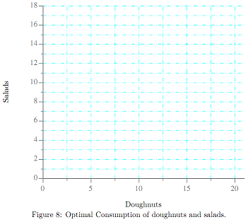
(h) Illustrate the solution by adding appropriate graphs to Figure 8. Briefly comment.

If the four marginality equations satisfy the hypotheses of the implicit function theorem, then these equations determine the optimal consumption bundle and Lagrange multipliers as functions of the prices and kilojoule content as well as the budgetary and dietary constraint values.

(i) Show that the four marginality equations satisfy the hypotheses of the implicit function theorem by showing the Jacobian computed with respect to the consumption of doughnuts and salads and the Lagrange multipliers is non-singular. Hint: You have most likely already computed the Jacobian and its determinant.

(j) Use the implicit function theorem to estimate the change in doughnut consumption resulting from a decrease in the in k_x from 15 to 12.

When economies of scale apply at all output levels relevant to a market a natural monopoly will often form. Preventing natural monopolies from forming will surely result in higher costs and may result in higher market prices. Society often prevents such enterprises from fully exploiting their monopoly status through regulation. Sometimes the regulation comes as a guaranteed return on investments made by the monopoly. The monopoly then makes profit maximizing investment decisions based on the returns negotiated with the regulators. Over capitalization may in some cases cause higher prices. The high retail electricity prices Australian consumers pay are often attributed to the "gold plating" of the electricity distribution network. The over capitalisation may even occur with publicly owned enterprises, see Nepal and Foster (2015).

In their 1962 article "Behavior of the Firm Under Regulatory Constraint" H. Averch and Johnson modelled the behaviour of regulated monopolies and provided a theoretical basis for over capitalisation. This phenomena has become known as the Averch-Johnson effect see H. A. Averch (2008).

Question 26 below provides a walk through of a version of the model used to illustrate the Averch-Johnson effect. The technique used is concave programming.

Q26. A firm wishes to maximize its economic profit

π(K, L) = E(K, L) - rK - wL.

Regulation prevents returns on capital expenditure exceeding a maximum rate so that

E(K, L) - wL ≤ mK.

Here, E gives earnings as a strictly concave twice continuously differentiable function of labour L and capital K, which is increasing in both labour and capital over their relevant ranges. Also, earnings are zero if either no labour or no capital is employed, E(0, L) = E(K, 0) = 0. The positive parameters r, w and m denote rent, wages and the maximum return to capital which is assumed to exceed rent so that m - r > 0.

(a) Determine the objective function and express the constraint as a function which must be non-negative.

(b) Briefly explain why the objective function is concave and the constraint function is convex.

(c) Write out the Lagrangian and Kuhn-Tucker conditions for this problem.

(d) Explain why the optimal value of the Lagrange multiplier, λ¯, cannot equal one.

(e) Given that the optimal values of capital and labour, K¯ and L¯ are both positive, use λ¯ ≠ 1 and the marginality equations to solve for the marginal revenue products of capital and labour, MRP_K = E_K and MRP_L = E_L.

(f) Briefly comment on the case where the constraint is non-binding.

(g) The Averch-Johnson effect occurs when greater than socially optimal levels of capital are employed in an enterprise. What values of the marginal revenue product of capital indicate the Averch-Johnson effect?

(h) What values of λ¯ are consistent with the Averch-Johnson effect?

If the return constraint is binding λ¯ > 0. The Kuhn-Tucker Sufficiency Theorem ensures that K¯, L¯ determines a profit maximum but does not ensure that λ¯ has a value that is consistent with the Averch-Johnson effect. The Kuhn-Tucker Sufficiency Theorem shows that K¯, L¯ and λ¯ provides unique solution to the equality constrained maximization problem,

Max π(K, L) = E(K, L) - rK - wL, subject to E(K, L) - wL = mK.

The second order sufficient condition involving the bordered Hessian provides an additional inequality which ensures a consistent value of λ¯.

(i) Write out the bordered Hessian corresponding to the constrained optimum above and then simplify using your result from 26e.

(j) By calculating appropriate determinants find an inequality which λ¯ must satisfy. Show that this inequality ensures that value of λ¯ is consistent with the Averch-Johnson effect.

Q27. Suppose that x^→₀ ∈ R³ satisfies the FONC for a constrained optimum with 2 constraints.

Objective: f(x^→) Constraints: g₁(x^→) = 0, g₂(x^→) = 0 Lagrangian: Z = f(x^→) - λ₁g₁(x^→) - λ₂g₂(x^→) and,

What conditions on H¯ ensure that x^→₀ determines a constrained local minimum? maximum?

Q28. Explain the differences between convex, concave, quasi-convex and quasi-concave functions.

Q29. Briefly say how quasi-convexity and quasi-concavity simplfy the sufficient conditions for a constrained optimum.

Attachment:- Assignment File.rar