Reference no: EM132366822
Assignment -
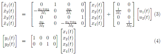
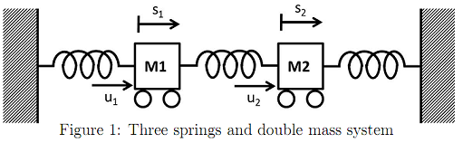
Question 1 - A three spring and double mass system is illustrated in Figure 1.
In this figure, the two blocks are with mass M1 and M2, and there are two spring constants α1 for the right and left springs, α2 for the middle spring. The manipulated variables are the two applied forces u1 and u2 and the output variables are the distances of the mass block movement y1 corresponding to block one and y2 corresponding to block two.
We consider the simplified spring force f1 where f1 = α1d1 and d1 is the distance of the mass movement, and apply Newton's law to the first block to obtain the following equation:
u1(t) - α1y1(t) - α2(y1(t) - y2(t)) = M1 (d2y1(t)/dt2) (1)
where the first term represents the first external force, the second and third terms represent the forces from spring 1 and spring 2, respectively. The right hand-side of (1) is the multiplication of the mass and acceleration of the block 1. Similarly, by applying Newton's law to the second block, we obtain
u2(t) - α1y2(t) + α2(y1(t) - y2(t)) = M2 (d2y2(t)/dt2) (2)
where the first term represents the second external force, the second and the third terms are the forces generated from spring 3 and spring 2. The right hand-side of (2) is the multiplication of mass and acceleration of the block 2. To convert these two equations into a state space model, two intermittent variables are chosen to reduce the second derivatives to first derivatives. Let x1(t) = y1(t), x2(t) = y·1(t) = x·1(t). Thus, x·2(t) = x¨1(t). Similarly, x3(t) = y2(t), and x4(t) = y·2(t) = x·3(t). Thus, x·4(t) = x¨3(t). The state space model is obtained as follows:
The physical parameters are M1 = 2kg, M2 = 4kg, α1 = 30N/m and α2 = 90N/m. The following tasks are completed by writing MATLAB programs.
1. Determine the eigenvalues of the spring-mass system.
2. Determine the controllability and observability of this system.
3. Design a state estimate feedback control system to stabilize this spring-mass plant using MATLAB place.m function where the closed-loop control system has poles at -3, -3.1, -3.2, -3.3 and the observer error system has poles -6, -6.1, -6.2, -6.3. (Note that we do not put integrators into the design because we only want to stabilize this system).
4. We assume that x1(0) = 0.5 and x3(0) = 0.1, x2(0) = x4(0) = 0, and xˆ1(0) = xˆ2(0) = xˆ3(0) = xˆ4(0) = 0. With sampling interval Δt = 0.001 (sec) and simulation time Tsim = 3 (sec), simulate the closed-loop response of the spring-mass system and present the responses of the four state variables in response to the initial conditions of system.
5. Where are the closed-loop poles for this state estimate feedback control system?
Question 2 - Assume that a dynamic system is described by the state space model
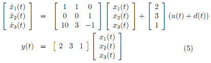
where the state variables x1(t), x2(t) and x3(t) are not measured and the input disturbance d(t) is an unknown constant. Design a state estimate feedback control system to follow a step reference signal r(t) = -1 and reject the constant input disturbance.
1. Here the closed-loop performance for the state estimate feedback control system is specified with the control system poles being located at -2±j0.5 and -3 and -3.2 and the observer poles being -5, -5.1 and -5.6.
2. With Δt = 0.001, and simulation time Tsim = 10 (sec) and the reference signal r(t) = -1, and disturbance d(t) = 3 that enters the simulation at half of the simulation time, simulate the closed-loop system response with initial state variable values at x1(0) = x2(0) = x3(0) = 2 and xˆ1(0) = xˆ2(0) = xˆ3(0) = 1. Present the closed-loop response of the output signal, and control signal for the reference following and disturbance rejection.
Question 3 - The mathematical model for the eighth reactor in a copolymerization reactor train is described by the following transfer function model:
Y(s) = [Ks + 1/τ21s2+2τ1τ2s+1]8 U(s) (6)
where the input is the flow rate of the Chain Transfer Agent (CTA) to the first reactor in the reactor train and the output is the weight-based average molecular weight (MWw). The parameters in the transfer function in the reactor start-up are given as K = 361.54, τ1 = 106.84 and τ2 = 1.72. Due to this system having a near pole-zero cancelation, the original mathematical model is not observable and controllable. We reduce the transfer function model from the 16th order to a third order model, which has the following form:
Y(s) ≈ (K/τ21)(1/(s + 0.0292)3) (7)
Based on this approximate model, design and simulate a state estimate feedback control system with integrator to control the reactor in the start-up phase.
1. Calculate the controller gain and the observer gain, where all the closed-loop controller poles are chosen to be -0.009 and all the observer poles are selected to be -0.09.
2. With reference signal r(t) = 1 and Δt = 3, simulate the closed-loop control responses and present the control signal and output signal. In the simulation, all initial conditions for the state variables and the estimated state variables are zero. Note that the chemical reactor has a slow response, choose the total simulation time to 3000 to try your simulation first. Increase the simulation time if it is not large enough.
3. Now, to demonstrate the strength of constrained control, choose a set of desired closed-loop performance that will lead to much faster responses. I suggest that you choose all the closed-loop controller poles to be -0.09 and all the observer poles to be -0.9. Because the system has a much faster response, you need to select a smaller sampling interval as Δt = 1. Simulate the closed-loop response from this much faster specification, and find the minimum and maximum values of the control signal from the previous step as uL and uU. We are only allowed to run the reactor within 80 percent of the flow rate for safety measure. Thus, we will let umin = 0.8uL and umax = 0.8uU. Now, imposing these constraints with anti-windup mechanism, simulate the closed-loop responses with r(t) = 1 and Δt = 3. Present the closed-loop control signal and output signal.
All simulation results must be submitted together with plots and printed MATLAB programs. Preferably, some discussions are given on your observations.