Reference no: EM133133727

FE545 Design, Patterns and Derivatives Pricing - Stevens Institute of Technology

Problem 1: Pricing a derivative security entails calculating the expected discounted value of its payoff. This reduces, in principle, to a problem of numerical integration; but in practice this calculation is often difficult for high-dimensional pricing problems. Broadie and Glasserman (1997) proposed the method of the simulated tree to price American options, which can derive the upper and lower bounds for American options. This combination makes it possible to measure and control errors as the computational effort increases. The main drawback of the ran- dom tree method is that its computational requirements grow exponentially in the number of exercise dates m, so the method is applicable only when m is small. Nevertheless, for problems with small m it is very effective, and it also serves to illustrate a theme of managing scoures of high and low bias.

Let h˜_i denote the payoff function for exercise at t_i, which we now allow to depend on i. Let V˜i(x) denote the value of the option at t_i given X_i = x_i (the option has not exercised). We are ultimately interested in V˜0(X₀). This value is determined recursively as follows:

V˜m(x) = h˜m(x)(1)

V˜_i-1(x) = max{h˜_i-1(x), E[D_i-1,i(X_i)V˜_i(X_i)|X_i-1 = x]}, (2)

i = 1, ..., m and we have introduced the notation D_i-1,i(X_i) for the discount factor from t_i-1 to t_i. It states that the option value at expiration is give by the payoff function h˜_m; and at time (i - 1)th exercise date the option value is the maximum of the immediate exercise value and the expected present value of continuing.

As its name suggests, the random tree method is based on simulating a tree of paths of the underlying Markov chain X₀, X₁, ..., X_m. Fix a branching parameter b ≥ 2. From the initial state X₀, simulate b independent successor states X₁, ..., X_b all having the law of X₁

From each X₁ⁱ, simulate b independent successors X₂ⁱ¹, ..., X₂^ib from the conditional law of X₂ given X₁ = X₁ⁱ. From each X₂ⁱ¹ⁱ², generate b successors X₃ⁱ¹ⁱ²¹, ..., X₃^i1i2b, and so on. We denote a generic node is the tree at time step i by X_i^j1j2...ji. The superscript indicates that this node is reached by following the j₁-th branch out of X₀, the j₂th branch out the next node, and so on.
At all terminal nodes, set the estimator equal to the payoff

at that node:

v_m^j1..jm = h_m(X_m^j1...jm ). (3)

At node j₁j₂...j_i at time step i, and for each k = 1, ..., b, set

v_ik^j1j2..ji = h_i(X_i^j1j2...ji)    if 1/b Σ^b_j=1 v_i+1^j1j2..jij ≤ _hi(X_i^j1j2....ji)

v_ik^j1j2..ji = v_i+1^j1j2..jik       Otherwise

then set

v_i^j1...ji = 1/bΣ^b_k=1 v_i,k^j1j2.

Working backword, we then set

v_i^j1...ji = max{h_i(X_i^j1..ji), 1/bΣ^b_k=1v_i,k^j1....ji.}

The high estimator of the option price at the current time and state is vˆ0.

The low estimator is defined as follows. At all terminal nodes, set the estimator equal to the payoff at that node:

v_i^j1j2...jm = h_m(X_m^j1j2...jm)

At node j₁j₂...j_i at time step i, and for each k = 1, ..., b, set

v_ik^j1j2..ji = h_i(X_i^j1j2...ji)    if 1/b Σ^b_j=1;j≠k v_i+1^j1j2..jij ≤ h_i(X_i^j1j2....ji)

v_ik^j1j2..ji = v_i+1^j1j2..jik       Otherwise

We then set

v_i^j1j2...ji = 1/bΣ^b_k=1 v_i,k^j1j2....ji

The low estimator of the option price at the current time and state is vˆ0.

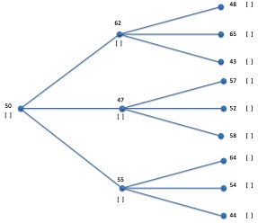
Figure 1: High Estimator

Assume a random tree for pricing American put option is given in Figure (1). Please use the random tree in Figure (1) to cal- culate the high and low estimate of the American call option price. Please show your steps for both the high estimator and low estimator.

Note: You do not need to write C++ program to get the price, but rather manually calculating the estimators following the algorithms introduced in class.

Problem 2: The Black-Scholes formula is sufficiently complicated that there is no analytic inverse function, and therefore this inversion must be carried out numerically. Our objective is to use Newton-Ralphson method and the programming techniques to design a solver in a reusable fashion.

When we have a well-behaved function with an analytic deriva- tive then Newton-Ralphson can be used to find inverse values of the Black-Scholes formula. The idea of Newton-Raphson is that we pretend the function is linear and look for the solution where the linear function predicts it to be. Thus we take a standing point x0, and approximate f by

g0(x) = f(x0) + (x - x0)fJ(x0).∈, (9)

We have that g0(x) equal to zero if and only if

x = (y - f (x0))/f'(x0) + x0

We therefore take this value as our new guess x1. We repeat until we find that f (x_n) is within s of y. In this problem, you will use a pointer to a member func- tion which is similar in syntax and idea to a function pointer, but it is restricted to methods of a single class. The difference in syntax is that the class name with a :: must be attached to the ∗ when it is declared. Thus to declare function pointers called V alue and Derivative which must point to methods of the class T , we have double (T::*Derivative) (double) double and double (T::*Value) (double) double. The function V alue (Derivative) is a const member function which takes in a dou- ble as argument and outputs a double as return value. If we have an object of class T called TheObject and y is a double, then the function pointed to can be invoked by either TheObject. ∗ V alue(y) or TheObject. ∗ Derivative(y). The following is the prototype of such a template class.
#include <cmath>

//three template parameters
template<class T, double (T::*Value)(double) const,double (T::*Deriv double NewtonRaphson(double Target,

double Start, double Tolerance, const T& TheObject)
{
double y = (TheObject.*Value)(Start); // pass initial guess to double x=Start;

while ( fabs(y - Target) > Tolerance )
{
double d = (TheObject.*Derivative)(x); x+= (Target-y)/d;
y = (TheObject.*Value)(x); // check the target function valu
}

return x;

}
Use the classes introduced in Lecture 09 and finish the main.cpp file for European Call Option with the following parameters:
• Expiry: 1
• Spot: 50
• Strike: 50
• Risk free rate: 0.05

• Dividend: 0.08
• Price: 4.23
• Vol initial guess: 0.23
• Tolerance: 0.0001
Use the NewtonRalphson class from the sample as the starting point and find implied volatility for the given option price of 4.23.

You are allowed to discuss the problems between yourselves, but once you begin writing up your solution, you must do so independently, and cannot show one another any parts of your written solutions.

Attachment:- Design, Patterns and Derivatives Pricing.rar