Reference no: EM132407993

Assignment - Multivariable Command Feed-forward for High Performance Drives with Resonant Loads

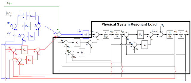
You are given the resonant load problem and asked to define an appropriate Command Feed-forward Structure to improve Command Tracking:

Definitions:

J₁ = 0.002 Kg-m²

K_lsa = 8.3 N-m/rad

b_r = 0.005 N-m/(rad/sec)

b_la = 0.36 N-m/(rad/sec)

K_r = 300 N-m/rad

b_ra = 1.97 N-m/(rad/sec)

K_ra = 0 N-m/rad

To do:

a. Design a command feed-forward controller assuming θ₁* and its derivatives are known. Evaluate the command following frequency response, θ₁/θ₁*, for the following cases:

1. All parameters are correctly estimated and b_ra = 0;

2. All parameters except for J₁ (varies from nominal to 3x) are correctly estimated and b_ra = 0;

3. All parameters are correctly estimated and b_ra = 1.97;

4. All parameters except for J₁ (varies from nominal to 3x) are correctly estimated and b_ra = 1.97;

b. Repeat Part a. assuming that position, velocity, and acceleration commands are known but higher order derivatives are not.

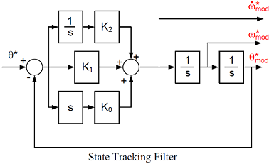
c. Assuming that you are not given the full command state vector, derive velocity and acceleration commands from the position command using the state tracking filter shown below. Tune the filter to have eigenvalues of 10 Hz, 100 Hz, and 1000 Hz. Explore the output of the tracking filter to sinusoidal inputs and step inputs.

d. Repeat Part b. using the modified position, velocity, and acceleration commands (output of the tracking filter) as the commands used to drive the resonant load system.

Hand in:

1. A derivation of the transfer functions and analysis (in the appendix).

2. Step Response and Frequency response plots showing the command tracking of the modified position command. For the step response, make three separate time domain plots (for modified position, modified velocity, and modified acceleration) for a step change in position command. For the sinusoidal response, plot using standard FRFs.

Calculate |θ*_mod/θ*|for each of the cases.

Amplitude (on linear scale) vs. frequency (on log scale).

Include your program listing with sufficient comments/text to allow reasonable review.

3. Frequency response plots showing the command tracking properties of the system for Parts a., b. and d.

Calculate |θ₁/θ₁*| for each of the cases.

Amplitude (on linear scale) vs. frequency (on log scale)

Include your program listing with sufficient comments/text to allow reasonable review.

4. Appropriately detailed discussion of important results and comparative findings.