Reference no: EM132164114
PROCESS MODELING AND SIMULATION
Q1. Neural networks have been used as an alternative to the traditional mathematical models to simulate complex patterns. The simplicity of their implementation makes them appropriate for modeling various complicated processes. Neural computing is largely motivated by the possibility of creating an artificial computing network similar to the brain and nerve cells in our body. Recent advances in neuroscience and in computers have sparked a renewed interest in neural network models for problem-solving.
Briefly describe about the techniques, structure, methodology, application and significance of Artificial Neural Networks (ANN) practiced in emerging areas of scientific research.
(Maximum 2000 words)
Q2. The following set of differential equations describes the change in concentration of three species in a tank. The reactions A→B→C occur within the tank. The constants k1, and k2 describe the reaction rate for A→B and B→C respectively.
The following ordinary differential equations (ode's) are obtained:
dCa/dt = -k1.Ca, dCb/dt = k1.Ca - k2.Cb, dCc/dt = k2.Cb
Where k1=1 hr-1, k2= 2 hr-1 and at time t=0, Ca = ......P........mol and Cb = Cc = 0 mol.
Solve the system of equations (using MATLAB) and plot the change in concentration of each species with respect to time. Select time interval for the integration as 0 ≤ t ≤ 5
Q3. The elementary irreversible liquid-phase reaction
A +B → C, - rA = kCACB
is carried out in a series of three identical CSTRs. The initial concentrations of A and B are CA0 = CB0 = 2 gmol/litre, the inlet flow rates of A and B are V0A = V0B = 6 litre/min , the reaction rate constant is k = 0.5, the volume of each reactor is V1 = V2 = V3 = 200 litre, and the flow rate of each stream is v1 = v2 = v3 = 12 litre/min.
Using MATLAB, plot the concentration of A exiting each reactor, CAi (i = 1, 2, 3), during start- up to the final time t = ...Q.....(0 ≤ t ≤ Q ).
Q4 Table 1 shows measurements of reaction temperature versus time for a chemical reaction in a Plug Flow Reactor. Using MATLAB determine the 1st-order, 2nd-order, and 4th-order polynomials to represent this data.
Table 1 : Reaction Temperature versus Time
|
t (hr)
|
1
|
2
|
3
|
4
|
5
|
6
|
7
|
R
|
|
T (ºC)
|
S
|
56.4
|
55.1
|
60.6
|
61.5
|
59.5
|
54.1
|
53.8
|
Also develop the regression equation for the 4th order polynomial model.
Q5 Figure 1 shows a series of three well-mixed tanks. From mass balance equations, we have
dV1/dt = q0 + m - q1
V1dx1/dt = q0 (x0 - x1) - mx1
V2dx2/dt = q1 (x1 - x1)
V3dx3/dt = q2 (x2 - x3)
where xi (i = 1, 2, 3) is the concentration (mol/liter) of the solution contained in the tank i. Under normal steady-state operation, m is maintained at 0 and qi (1, 2, 3) is kept constant.
At a certain time (t = 0), m is suddenly increased to 12 liter/min. Using MATLAB plot the concentrations in the three tanks from t = 0 to ...T...... The initial conditions are x0 = 0.15 mol/liter and q0 = 15 liter/min, and the initial volume of each tank is 20 liter.
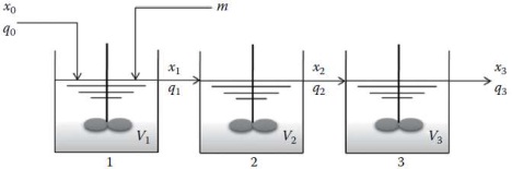
Figure 1
Attachment:- Process Modeling and Simulation.rar