Describe the diurnal variation of cloud

Assignment Help Python Programming

Reference no: EM132291653

Homework - Data fitting

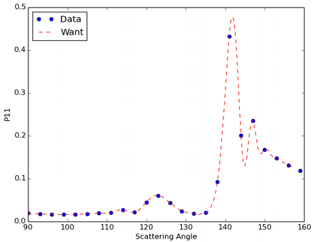
Problem 1 - So far in the Monte-Carlo radiative transfer code, we have been using the isotropic scattering phase function. The figure below shows the scattering phase function of water droplet for the scattering angle between 90~160 degree.

Now, suppose that you have obtained the scattering phase function at some coarse resolution (i.e., the blue dots in the figure). Use the 1) linear, 2) Lagrange and 3) cubic spline methods to interpolate and get high-angular resolution data at every 0.5 degree.

The data needed for this problem are in the .npy file. Use the Numpy.load function to load the data.

X_low = np.load(work_path+'scattering_angle_low.npy')

Y_low = np.load(work_path+'Phase_function_low.npy')

X_high = np.load(work_path+'scattering_angle_high.npy')

Y_high = np.load(work_path+'Phase_function_high.npy')

Where the work path is the working directory where you saved the data.

Problem 2 - Assume your Monte-Carlo radiative transfer code computes the cloud reflectances ("Ref") for several values of cloud optical thickness ("Tau"). See data below.

1) Use cubic spline method the interpolate the data.

2) Use the model Ref = Tau/(a+bTau) to fit the data, where a and b are two adjustable parameters. Find the optimal values for a and b.

3) Convert the second problem to a linear fitting problem.

Tau = np.array([ 0.299, 1.29400003 , 2.28900003 , 3.28399992, 4.27899981, 5.27399969 , 6.26900005 , 7.26399994, 8.25900078 , 9.25400066, 10.2490005, 11.2440004 , 12.2390003, 13.2340002 , 14.2290001, 15.2240009 , 16.2189999 , 17.2140007 ,18.2089996 , 19.2040005 ])

Ref = np.array([ 0.17678887, 0.48721159 , 0.62823123 , 0.70785129, 0.75912076, 0.79498094, 0.82153791, 0.84198004, 0.85822612, 0.87143803, 0.8823905, 0.89163792, 0.89952338, 0.90634716, 0.91229314 , 0.91752762, 0.92218465, 0.92633438, 0.93006754, 0.93343675])

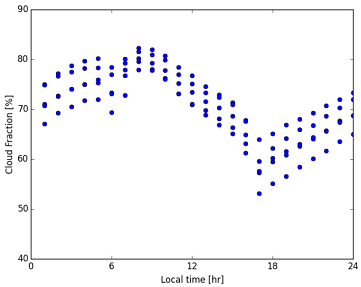
Problem 3 - The file "Cloud_Fraction.npy" contains 4 years satellite observations of the diurnal variation of cloud fraction in the Southeast Atlantic region. As you can see, the cloud fraction has a strong diurnal cycle. This is primarily because increasing solar radiation leads to stronger cloud absorption that "burns" off cloud fraction.

Based on the cloud fraction data, develop a non-linear model to describe the diurnal variation of cloud in the Southeast Atlantic region. Print out the formula of your model and list all adjustable parameters. Plot the fitting result in the same figure with the original data.

To read the cloud fraction data use the command: cf = np.load('Cloud_Fraction.npy')

Note - Need help with this assignment in python 3.

Attachment:- Assignment Files.rar

Reference no: EM132291653

Questions Cloud

Advertising their products except : Companies do all of the following while advertising their products EXCEPT:

How can we analyze the parts of cultural intelligence : Recall how understanding cultural differences is more than identifying with diversity. How can we analyze the parts of cultural intelligence?

Give four reasons and explain why a command economy : Give four reasons and explain why a Command Economy, like the one found in China, could be a good option for the United States.

Discuss what conclusions can be drawn : Write an analytic essay in which you explore what both authors' works, when put side by side, say about a specific topic - discuss what conclusions can be drawn

Describe the diurnal variation of cloud : Homework - Data fitting Based on the cloud fraction data, develop a non-linear model to describe the diurnal variation of cloud in the Southeast Atlantic region

Discuss what factors have provided motivation : Discuss what factors have provided motivation for you to do your best work. Discuss what factors have discouraged you from doing your best work.

Why globalization could be a contributor to global warming : Give four reasons and explain why globalization could be a contributor to Global Warming.

Smaller widths are to be cut from larger standard size reel : 120 reels of 20-inch width; and (iii) 80 reels of 12-inch width. These smaller widths are to be cut from the larger standard size reel.

Prevent an ethical challenge like this from arising again : What specific steps (e.g., change in systems, policies, etc.) would you recommend a company take to either prevent an ethical challenge like this from arising

Reviews

len2291653

4/23/2019 9:52:33 PM

Instructions: I need help with this assignment in python 3. I need it to be as simple as possible and well commented. I will attach all the files needed along with the description. Use the 1) linear, 2) Lagrange and 3) cubic spline methods to interpolate and get high-angular resolution data at every 0.5 degree.

Write a Review

Required(*) Message

User Account

All Pages