Reference no: EM133508411

Control of Mechatronic Systems

Question 1:

Examine the state space model of the inverted pendulum in Figure 1 and answer the following questions. Click the following link to find the state space model (for reference only):

Assume that:

(Vc) volume of the aluminium cart  2000cm³
(Vp) volume of the aluminium pendulum 600cm³
(ρ) density of the aluminium 2.7g/cm³
(b) friction of the cart 0.5 N/m/s
(l) length to pendulum 0.3 m
(I) inertia of the pendulum 0.01 kg*m²
(F) force applied to the cart
(x) cart position coordinate
(θ) pendulum angle from vertical

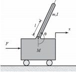
Figure 1. Inverted Pendulum

(1) Check the stability and the observability of the system.
(2) Design state feedback control law u = -Kx such that the poles of the closed-loop system are -4, -3, -5, -7. Show the state trajectory and output trajectory in MATLAB for a given initial state.

Question 2:

Consider the mechanical system given in Figure 2. d₁(t) and d₂(t) are the displacements of the two blocks with respect to their nominal positions (when no any force exist). v₁(t) and v₂(t) are the velocities of the two blocks, respectively.

 

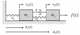
Figure 2. Mechanical System

An external force f(t) is applied to the system as the input. Assume that the movement of blocks 1 and 2 is opposed by viscous friction forces given by
fD₁ (t) = D₁v₁(t), fD₂ (t) = D₂v₂(t)

Choose the state vector to be

X(t) = [d₁(t) d₂(t) v₁(t) v₂(t)]^T

(1) Derive the state-space model of the system. Assume the output of the system, y(t), is the velocity of the second block.
(2) Analyse the stability, controllability and observability of the system. Assume the parameters are given by:

M₁ = 4 [kg] , M₂ = 8 [kg], k₁ = 20 [Nm-1], k2 = 30 [Nm-1],
b = 10 [Nsm-1], D₁ = 6[Nsm-1], D2 = 8[Nsm-1]

(3) Design state feedback control law u = -Kx such that the poles of the closed-loop system are -3, -11, -12, -16. Show the state trajectory and output trajectory in MATLAB for a given initial state.

(4) Next, choose the state vector as

X‾(t) = [d1(t) d2(t) - d1(t) v1(t) v2(t) - v1(t)]^T

Apply similarity transformation to obtain the new state space model using the new state vector. Analyse the stability, controllability and observability of the new system.

Question 3:

A linear continuous time system is given by a state space model with

Without using MATLAB, analysing the following properties of the above system for all the possible real number ????

(1) Asymptotic stability
(2) Controllability
(3) Observability

Question 4:
Formulate the mobile robot trajectory following problem as a control problem. A mobile robot position at time t is denoted as (K(t), y(t)) and its orientation at time t is denoted as θ(t), the velocity and turn rate are denoted as v(t) and ω(t) respectively. The nonlinear motion model can be simplified as

x^· = v cos θ , y^· = v sin θ , θ^· = ω.

Suppose the desired trajectory is

x^~(t) = 5t, y^~ (t) = 5t, θ^~(t) = Π/4.

Assuming v(t) is close to 5√2m/s, ω(t) is close to 0 and θ(t) is close to Π/4, define the difference between the actual trajectory and the desired trajectory as the state, v(t) - 5√2 and ω(t) as control inputs, assume the output is the same as the state, derive the state-space model of the linearized control system.