Reference no: EM132506224

Process-Control Assignment - Answer all three questions.

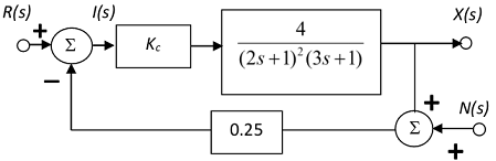
Q1. Consider the block diagram shown below. The third order process shown is controlled by a simple proportional controller. What range of permitted values for the proportional gain K_c may be employed? Estimate the percentage offset in the response signal that would be observed for a unit step change in the set-point if the maximum allowed value for the proportional gain was employed (note that sN(s) → 0 as s → 0). Outline briefly a technique for plotting the root locus for this system.

(b) In a process, the first-order irreversible reaction

A → B

takes place in a CSTR. The concentration of product B in the reactor is controlled by adjusting the flow-rate of the reactant stream (pure A) entering the reactor. The control scheme is a two-level cascade with a reactant A concentration controller linked to the reactor exit and a flow controller on the feed stream. The resulting block diagram with unity feedback in both the primary and slave loops is shown below.

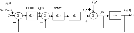
The valve transfer function is modelled as first order lead-second order lag (with s in units of min^-1)

G_v(s) = (1-s)/(1+s)²

and the reactor transfer function (linearised with respect to the steady-state flowrate F_SS and steady-state product concentration c_A,SS) is

G_R(s) = K/(τs+1) with K = F_SS/(F_SS+kV) = 0.5 and τ = V/(F_SS+kV) = 6 min

Note that the reactor transfer function is explicitly

G_R(S) = C_A(s)/F*(s)

where F* = Fc_A,IN/F_SS and c_A,IN is the inlet molar concentration of the reactant vis-à-vis the steady-state effluent concentration.

If FC102 is a proportional controller with gain K_c2 and CC101 is a PI controller with gain K_c1 and integral time τ_I then, using the controller settings for closed-loop tuning provided by Ziegler and Nichols:

(i) Specify K_c2 for the slave loop.

(ii) Verify that the ultimate frequency for the master loop is 1.074 rad.min^-1, and specify K_c1 and τ_I for this loop.

Q2. A process has the transfer function

G(s) = Kexp(-Ts)/(τ_ps+1)

where K, T and τ_p have nominal values of 1.0, 2.0 minutes and 5.0 minutes, respectively, and the control loop has unity feedback.

(i) Develop the controller transfer function and the settings to be used in this control loop using the Controller Synthesis Formula with τ_c = 5 minutes in the closed loop transfer function

X(s)/R(s) = exp(-Ts)/τ_cs+1

Note that in generating the expression for G_c(s), you may use the Padé approximant

exp(-Ts) ≈ (1-(T/2)s)/(1+(T/2)s)

(ii) For a long dead time and 'tight' control, derive the effective type (or mode) of controller to be used, along with expressions for its key properties, such as gain and appropriate time constant(s).

(iii) Suppose that the controller settings found in (i) are employed and that the process gain, K, changes unexpectedly from 1.0 to 1.0 + α without change in the synthesised controller settings. For what values of α will the closed-loop system be stable?

(b) Consider a feedback control loop consisting of unity feedback along with a simple first-order process subject to a dead (delay) time. For a proportional controller, derive an expression for the maximum allowable controller gain in terms of dead and process times, subject to the dead time being much smaller than the characteristic (or relaxation) time of the process itself.

Q3. A continuous process consists of two sections, A and B, shown in the figure below. Feed of composition X₁ enters section A where it is extracted with a solvent pumped at a rate L₁ to A. The raffinate stream is removed from A at a rate L₂, whilst the extract is pumped to a cracking section B. Hydrogen is added at the cracking stage at a rate L₃ whilst heat is supplied at a rate Q. Two products are formed, having compositions X₃ and X₄. The feed rate to A, along with L₁ and L₂, can be kept constant easily, but it is known that fluctuations in X₁ can occur. Consequently, a feed-forward control system is proposed to keep X₃ and X₄ constant vis-à-vis variations in X₁, using L₃ and Q as controlling variables. Experimental frequency-response analysis yielded the following transfer functions:

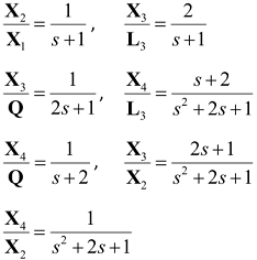
where X₁, X₂, L₃, Q, etc. denote the Laplace transforms of small time-dependent perturbations, i.e., deviations about steady-state, in the variables X₁, X₂, L₃, Q.

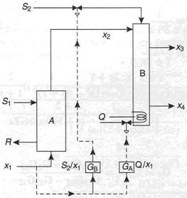
Determine the transfer functions of the feed-forward control scheme, assuming linear operation and negligible distance-velocity lags throughout the process. Comment on the stability of the feed-forward controllers which you specify.