Reference no: EM132569451

ENGI 7854 Image Processing and Applications - Memorial University of Newfoundland

Introduction

The objective of this laboratory exercise is to get familiarized with frequency domain filtering concepts.

Frequency Domain Procedure Review

The frequency domain image filtering process can be performed as follows:
1. Given the input image f (x, y) of size M × N , obtain the padding sizes P = 2M and Q = 2N .
2. Form a padded image of size P × Q using zero padding.
3. Multiply f (x, y) by (-1)^x+y to centre the Fourier transfrom (FT) on the P × Q frequency rectangle.
4. Compute the DFT, F (u, v) of the centred image
5. Construce a real, symmetric filter transfer function, H(u, v), of size P × Q with centre at (P/2, Q/2).
6. Form the product G(u, v) = H(u, v)F (u, v) using element-wise multiplication.
7. Obtain the Inverse Fourier transform of G(u, v), ignoring parasitic complex components:
g_p(x, y) = (real[F^-1G(u, v)])(-1^x+y)

8. Obtain the final result, g(x, y), of the same size as the input image by extracting the M × N region from the top left quadrant of gp(x, y).

Note that centering the transform helps to visualize the filtering process and to generate the filter functions, but centering is not a fundamental requirement.

Part 1: Low pass and High pass filter design

1. Download the test image (puppy.jpg) and lp hp filters.m from D2L under Lab 3 and save it in the MATLAB working directory. Read the file and understand the implementation.

2.Read the image and convert the image to a grayscale image. Obtain the padding parameters and FT the image.

F_rgb=imread('puppy.jpg'); % read the gs image
F=rgb2gray(F_rgb);
im_size=size(F); % Obtain the size of the image
P=2*im_size(1);Q=2*im_size(2); % Optaining padding parameters
as 2*image size
FTIm=fft2(double(F),P,Q); % FT with padded size

3. Design the ILPF
D0 = 0.1*im_size(1); %Cutoff freqency radius is 0.1 times the
the hight of the image
n=0; %For use only in Butterworth filters. For BTW filters,
Order(n)>0
%Filter_type=('ideal' or 'btw' or 'gaussian')
%lp_or_hp=('lp' or 'hp' for low pass or high pass),
Filter = lp_hp_filters('ideal','lp', P, Q, D0,n); % Calculate
the LPF
4. Implement the filter by multiplying the FT of the image with filter. Undo padding.
Filtered_image=real(ifft2(Filter.*FTIm)); % multiply the FT of
image by the filter and apply the IDFT
Filtered_image=Filtered_image(1:im_size(1), 1:im_size(2)); %
Resize the image ( undo padding)

5. Move the origin of frequency spectrum to the center and display the results

Fim=fftshift(FTIm); % move the origin of the FT to the center

display)
subplot(2,2,1), imshow(F,[]), title('Original Image'); % show
the image
subplot(2,2,2), imshow(FTI,[]), title('FT of Original'); %
show the image
subplot(2,2,3), imshow(FTF,[]), title('Filter in frequency
domain'); % filter
subplot(2,2,4), imshow(Filtered_image,[]), title('Filtered
Image'); % show the image

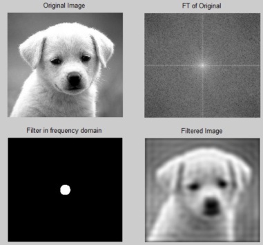
Figure 1: Result of ILPF the image

Part 2

1.Implement an Ideal low pass filter for cutoff frequencies (0.3 and 0.7 of image height). 2.Implement a Butterworth low pass filter for cutoff frequencies (0.1 and 0.5 of image height) and order n = 1, 5, 20.
3. Implement a Gaussian low pass filter for cutoff frequencies (0.1, 0.3 and 0.7 of image height) .
4. Implement an Ideal high-pass filter for cutoff frequencies (0.1, 0.3 and 0.7 of image height). 5.Implement a Butterworth high pass filter for cutoff frequencies (0.1 and 0.5 of image height) and order n = 1, 5, 20.
6.Perform a Gaussian high pass filtering for cutoff frequencies (0.1, 0.3 and 0.7 of image height).

Discussion

1. What can you observe when increasing the cut off frequency radius of the Ideal filter?

2. What can you observe when increasing the order of the Butterworth filter when the cut-off frequency remains the same?

3. Discuss the general performance of the Gaussian filters in comparison to the Ideal and Butterworth filters. You do not need to discuss each possible comparison case. Only discuss any interesting phenomenon or performance observations.

Note: Include your MATLAB code in your lab report along with your results.