Reference no: EM132394157

Assignment

In all cases, include your functions and an example run in your submission. Please submit your document (PDF, docx, etc.) and your Python file.

1 Question

Write a new function Spring3 which is a modified version of Spring2. It will take two inputs, the number of iterations and the spring constant k. The output is a tuple of two variables: the position and velocity for the last iteration.

The constants you will use inside the function Δx = 0:5, m = 1, v₁ = 0 and Δt = 0:1.

Run the function with k = 0:5 and print out the position and velocity after 12 iterations.

2 Question

Run the function created in the previous question. The only change is that the value of k is doubled. What is the position and velocity after 12 iterations?

3 Question

The potential energy of a mass oscillating on a spring is:

U = 1/2(kΔx²).

This measures the energy stored up in the system. The spring has more potential energy when the spring is compressed or stretched. Create a new function named Spring4 which is a modified version of Spring3.

The only change is that it has a list which collects the potential energy after each iteration. The output of Spring4 is only this list.

Run your function for 500 iterations, with k = 0:5. Use the following code to create a plot from the list created by Spring4 where potEnergyList is the output list from Spring4. Copy the plot to your homework document along with the code.

1 import matplotlib . pyplot as plt

2 plt . plot ( potEnergyList )

4 Question

The kinetic energy measures the energy of a moving mass. The equation is K = 1/2(mv²):

Modify Spring4 to also capture the values of the kinetic energy. Now, the function will return two lists. The first is the potential energy and the second is the kinetic energy. Use the same code above, for the same number of iterations and k-value to create a plot for the kinetic energy.

5 Question

The total energy is the sum of the potential energy and kinetic energy. Modify Spring4 once more. A third list collects the total energy for each iteration. Now, the function returns the potential energy list, the kinetic energy list, and the total energy list. Run the function with the same values as before and create a plot of the data collected in the total energy list.

6 Question

Without friction the spring will oscillate forever. So, we will add friction to slow it down. Friction affects the calculation of velocity. After you have calculated v2, multiply it by 0.99. This will reduce the velocity a little bit in each iteration, thus behaving somewhat like friction.

Create a new function named Spring5 which is much like the previous function. Do not collect the energies in this function. Instead, collect the position of the mass at each iteration. Plot the position values collected in this list.

7 Question

Recall the equation for an object under the influence of gravity,

y₂ = y₁ + v₁Δt + (1/2) gΔt²;

where g = −9:8. Recall also that the quadratic formula was used to compute the time of flight for this system.

Write a Python script to compute the time of flight for the object dropped from a height of 5 m. The computation of this time will return values. Keep the only one that makes sense.

8 Question

Compute the height of a following object at each time step. The starting height is h = 5 m, gravity is g = −9:8 m=s², and the time step is Δt = 0:1 sec Recall the equation for the change of velocity for an object under the influence of gravity,

v₂ = v₁ + gΔt.

Write and use a Python function named Drop1. This function will collect values of height in a list. Inside of your loop, compute the following:

1. Compute the new velocity using the equation above.

2. Compute the new height using the equation in the previous problem.

3. Put the value for the new height in a list.

4. Assign the value of the new height h₂ to the old height h₁.

5. Assign the value of the new velocity v₂ to the old velocity v₁.

Create a plot of the height values in the list.

9 Question

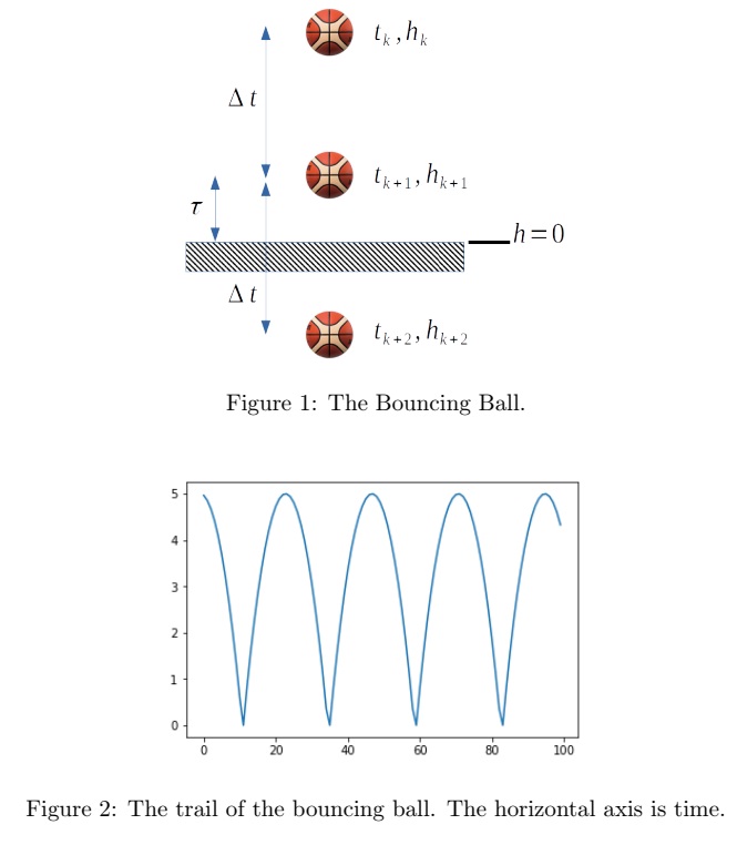
Add bounce to your program. Create a new program named Drop2 which is a modified version of Drop1. It has one change. Consider Figure 1. The ball is dropping and at a time tk it is at a height hk. The next time step ?t brings the ball to a new height h_k+1. The equations from the previous problem will work for this time step.

The next time step, brings the ball to a new height h_k+2 which is below the floor. It order to simulate the bounce, the computation must be stopped at the floor. So, the program needs to be modified. If the ball is in the last time step before hitting the floor:

• Compute τ, the time it takes to go from h_k+1 to the floor. See Question 7.

• Replace Δt with τ in the equations. Compute the velocity when the ball hits the floor.

• Define the bounce as simply reversing the sign on the velocity when the object is on the floor.

Run your simulation for 100 iterations. Plot the heights. The result should look something like Figure 2.
(Figure 2 uses different parameters and so your answer will not look exactly like this one.)

10 Question

Write a new Python function named Drop3. It is the same as the previous problem except friction is added to the simulation. After the calculation of each iteration, multiply v₂ by 0.99. Create a new graph of the bouncing ball.