Reference no: EM132023

Exercise 1 (Jacobi and Gauss-Seidel Iterations) Consider the following linear system

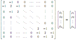
This is a discrete version of Poisson's equation: ΔΦ = ρ
 = , which may be written in partial derivatives as ∂²Φ/∂x² = ρ. Poisson's equation is ubiquitous in physics, arising in electrostatics (Φ is the electric potential and -ρ is the charge density), in gravitation (Φ is the gravitational potential and ρ is the mass density), in uid dynamics (Φ is the velocity and ρ is the negative curl of vorticity), etc. It is also important in image analysis. We will see how this relates to the above matrix equation later in the course.

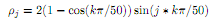
Construct the A matrix above for a 49 x 49 system. Use the >> help diag command for information about constructing a tridiagonal matrix in MATLAB. Set k = 45 and construct a (rho) vector according to the following rule:

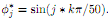
Verify that the solution Φ* (phistar) that satis es AΦ* = ρ is given by

Now, program both the Jacobi and Gauss-Seidel methods for solving this problem, and in each case, start the iterations with an initial guess Φ as a column of ones. Continue to iterate each method until every term in the vector Φ converges to within 10^-4 of the same term in the previous iteration (this corresponds to norm(phi(:,k+1)-phi(:,k),Inf)<=1.e-4.).

Exercise 2 Consider the following graph representing the probability of the weather tomorrow, given the weather today.

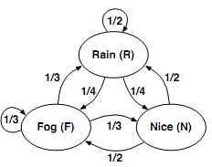
We may represent these probabilities in a Markov matrix, leading to the following equation:

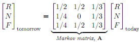
More concisely, we may write

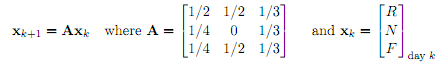
(a) Compute the eigenvalues and eigenvectors of the matrix A using the eig command. Rear-range the eigenvalues as a single column vector (hint: use the diag command).

Exercise 3: Consider the following temperature data taken over a 24-hour (military time) cycle:

75 at 1, 77 at 2, 76 at 3, 73 at 4, 69 at 5, 68 at 6, 63 at 7, 59 at 8, 57 at 9, 55 at 10, 54 at 11,52 at 12, 50 at 13, 50 at 14, 49 at 15, 49 at 16, 49 at 17, 50 at 18, 54 at 19, 56 at 20, 59 at 21, 63at 22, 67 at 23, 72 at 24.

(a) Fit the data with the parabolic fi t

f(x) = Ax² + Bx + C

and calculate the E₂ error. Use polyfit and polyval to get your results. Evaluate the curve f(x) for x = 1 : 0:01 : 24 and save this in a column vector.