Reference no: EM132246139
Applied Statistics Assignment -
Q1. Determine whether the scatter diagram indicates that a linear relation may exist between the two variables. If the relation is linear, determine whether it indicates a positive or negative association between the variables.
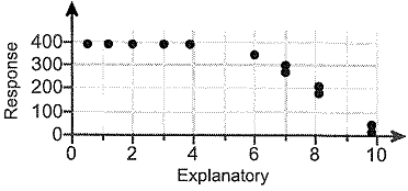
Use this information to answer the following.
Do the two variables have a linear relationship?
A. The data points do not have a linear relationship because they lie mainly in a straight line.
B. The data points have a linear relationship because they lie mainly in a straight line.
C. The data points have a linear relationship because they do not lie mainly in a straight line.
D. The data points do not have a linear relationship because they do not lie mainly in a straight line.
If the relationship is linear do the variables have a positive or negative association?
A. The variables have a positive association.
B. The variables have a negative association.
C. The relationship is not linear.
Q2. Determine whether the scatter diagram indicates that a linear relation may exist between the two variables. If the relation is linear, determine whether it indicates a positive or negative association between the variables.
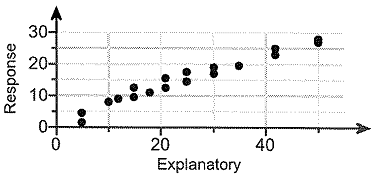
Use this information to answer the following.
Do the two variables have a linear relationship?
A. The data points have a linear relationship because they do not lie mainly in a straight line.
B. The data points do not have a linear relationship because they do not lie mainly in a straight line.
C. The data points have a linear relationship because they lie mainly in a straight line.
D. The data points do not have a linear relationship because they lie mainly in a straight line.
Do the two variables have a positive or a negative association?
A. The two variables have a positive association.
B. The two variables have a negative association.
C. None of the above.
Q3. For the accompanying data set, (a) draw a scatter diagram of the data, (b) compute the correlation coefficient, and (c) determine whether there is a linear relation between x and y.
Data set
Critical values for the correlation coefficient
|
n
|
|
|
3
|
0.997
|
|
4
|
0.950
|
|
5
|
0.878
|
|
6
|
0.811
|
|
7
|
0.754
|
|
8
|
0.707
|
|
9
|
0.666
|
|
10
|
0.632
|
|
11
|
0.602
|
|
12
|
0.576
|
|
13
|
0.553
|
|
14
|
0.532
|
|
15
|
0.514
|
|
16
|
0.497
|
|
17
|
0.482
|
|
18
|
0.468
|
|
19
|
0.456
|
|
20
|
0.444
|
|
21
|
0.433
|
|
22
|
0.423
|
|
23
|
0.413
|
|
24
|
0.404
|
|
25
|
0.396
|
|
26
|
0.388
|
|
27
|
0.381
|
|
28
|
0.374
|
|
29
|
0.367
|
|
30
|
0.361
|
(1) positive
negative
(2) greater
not greater
(3) no
a positive
a negative
(a) Draw a scatter diagram of the data. Choose the correct graph below.
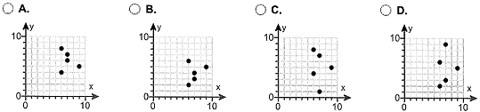
(b) Compute the correlation coefficient.
(c) Determine whether there is a linear relation between x and y.
Because the correlation coefficient is (1) ______ and the absolute value of the correlation coefficient, _______ , is (2) ________ than the critical value for this data set, _______ , (3) ________ linear relation exists between x and y.
Q4. The data in the table to the right are based on the results of a survey comparing the commute time of adults to their score on a well-being test.
|
Commute Time (in minutes)
|
Well-Being Score
|
|
7
|
69.4
|
|
15
|
68.4
|
|
23
|
67.6
|
|
34
|
67.5
|
|
53
|
66.1
|
|
66
|
65.5
|
|
95
|
63.5
|
Critical value for Correlation Coefficient
|
n
|
|
|
3
|
0.997
|
|
4
|
0.950
|
|
5
|
0.878
|
|
6
|
0.811
|
|
7
|
0.754
|
|
8
|
0.707
|
|
9
|
0.666
|
|
10
|
0.632
|
|
11
|
0.602
|
|
12
|
0.576
|
|
13
|
0.553
|
|
14
|
0.532
|
|
15
|
0.514
|
|
16
|
0.497
|
|
17
|
0.482
|
|
18
|
0.468
|
|
19
|
0.456
|
|
20
|
0.444
|
|
21
|
0.433
|
|
22
|
0.423
|
|
23
|
0.413
|
|
24
|
0.404
|
|
25
|
0.396
|
|
26
|
0.388
|
|
27
|
0.381
|
|
28
|
0.374
|
|
29
|
0.367
|
|
30
|
0.361
|
Complete parts (a) through (d) below.
(a) Which variable is likely the explanatory variable and which is the response variable?
A. The explanatory variable is commute time and the response variable is the well-being score because well-being score affects the commute time score.
B. The explanatory variable is the well-being score and the response variable is commute time because well-being score affects the commute time.
C. The explanatory variable is the well-being score and the response variable is commute time because commute time affects the well-being score.
D. The explanatory variable is commute time and the response variable is the well-being score because commute time affects the well-being score.
(b) Draw a scatter diagram of the data. Which of the following represents the data?
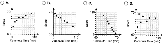
(c) Determine the linear correlation coefficient between commute time and well-being score.
(d) Does a linear relation exist between the commute time and well-being index score?
A. Yes, there appears to be a positive linear association because r is positive and is greater than the critical value.
B. Yes, there appears to be a negative linear association because r is negative and is less than the negative of the critical value.
C. No, there is no linear association since r is positive and is less than the critical value.
D. Yes, there appears to be a positive linear association because r is positive and is less than the critical value.
Q5. Lyme disease is an inflammatory disease that results in a skin rash and flulike symptoms. It is transmitted through the bite of an infected deer tick. The following data represent the number of reported cases of Lyme disease and the number of drowning deaths for a rural county.
Data table -
|
Cases of Lyme Disease
|
Drowning
Deaths
|
Month
|
|
3
|
0
|
J
|
|
1
|
1
|
F
|
|
3
|
2
|
M
|
|
4
|
1
|
A
|
|
5
|
3
|
M
|
|
15
|
9
|
J
|
|
22
|
16
|
J
|
|
13
|
5
|
A
|
|
6
|
3
|
S
|
|
5
|
3
|
0
|
|
4
|
1
|
N
|
|
1
|
0
|
D
|
View the critical value table in Q3.
Complete parts (a) through (c) below.
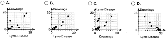
(a) Draw a scatter diagram of the data. Choose the correct graph below.
(b) Determine the linear correlation coefficient between Lyme disease and drowning deaths.
(c) Does a linear relation exist between the number of reported cases of Lyme disease and the number of drowning deaths?
Because the correlation coefficient is (1) ______ and the absolute value of the correlation coefficient, ______ , is (2) ______ than the critical value for this data set, ______, (3) ______ linear relation exists between Lyme disease and drowning deaths. (Round to three decimal places as needed.)
Do you believe that an increase of Lyme disease causes an increase in drowning deaths? What is a likely lurking variable between cases of Lyme disease and drowning deaths?
A. An increase in Lyme disease does not cause an increase in drowning deaths. There are no lurking variables.
B. An increase in Lyme disease does not cause an increase in drowning deaths. Pesticide control and life guards are likely lurking variables.
C. An increase in Lyme disease does not cause an increase in drowning deaths. The temperature and time of year are likely lurking variables.
D. An increase in Lyme disease causes an increase in drowning deaths. There are no lurking variables.
Q6. A data set is given below.
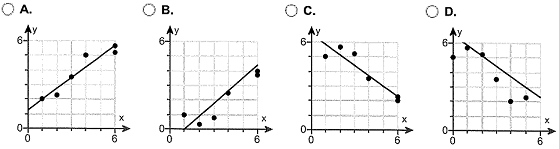
(a) Draw a scatter diagram. Comment on the type of relation that appears to exist between x and y.
(b) Given that x- = 3.6667, sx = 2.0656, y- = 3.9500, sy = 1.5783, and r = -0.9264, determine the least-squares regression line.
(c) Graph the least-squares regression line on the scatter diagram drawn in part (a).
|
x
|
1
|
2
|
3
|
4
|
6
|
6
|
|
y
|
5.0
|
5.7
|
5.2
|
3.5
|
2.0
|
2.3
|
(a) Choose the correct graph below.
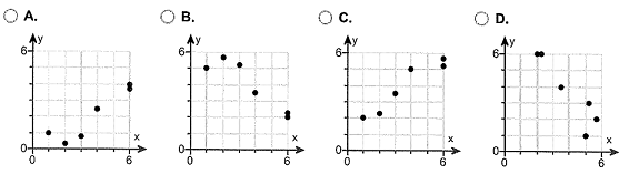
There appears to be (1) ______ relationship.
(b) y^ = _______ x + (_______) (Round to three decimal places as needed.)
(c) Choose the correct graph below.
Q7. An engineer wants to determine how the weight of a gas-powered car, x, affects gas mileage, y. The accompanying data represent the weights of various domestic cars and their miles per gallon in the city for the most recent model year.
Car Weight and MPG
|
Weight
(pounds), x
|
Miles per
Gallon, y
|
|
3786
|
18
|
|
3923
|
17
|
|
2814
|
25
|
|
3459
|
19
|
|
3225
|
22
|
|
2942
|
23
|
|
3632
|
18
|
|
2575
|
23
|
|
3518
|
18
|
|
3853
|
16
|
|
3353
|
19
|
Complete parts (a) through (d) below.
(a) Find the least-squares regression line treating weight as the explanatory variable and miles per gallon as the response variable.
(b) Interpret the slope and y-intercept, if appropriate. Choose the correct answer below and fill in any answer boxes in your choice. (Use the answer from part a to find this answer.)
A. A weightless car will get _______ miles per gallon, on average. It is not appropriate to interpret the slope.
B. For every pound added to the weight of the car, gas mileage in the city will decrease by _______ mile(s) per gallon, on average. A weightless car will get _______ miles per gallon, on average.
C. For every pound added to the weight of the car, gas mileage in the city will decrease by _______ mile(s) per gallon, on average. It is not appropriate to interpret the y-intercept.
D. It is not appropriate to interpret the slope or the y-intercept.
(c) A certain gas-powered car weighs 3700 pounds and gets 20 miles per gallon. Is the miles per gallon of this car above average or below average for cars of this weight?
(d) Would it be reasonable to use the least-squares regression line to predict the miles per gallon of a hybrid gas and electric car? Why or why not?
A. Yes, because the absolute value of the correlation coefficient is greater than the critical value for a sample size of n =11.
B. Yes, because the hybrid is partially powered by gas.
C No, because the hybrid is a different type of car.
D. No, because the absolute value of the correlation coefficient is less than the critical value for a sample size of n = 11.
Q8. Because colas tend to replace healthier beverages and colas contain caffeine and phosphoric acid, researchers wanted to know whether cola consumption is associated with lower bone mineral density in women. The accompanying data lists the typical number of cans of cola consumed in a week and the femoral neck bone mineral density for a sample of 15 women.
Data Table -
|
colas per week
|
Bone Mineral Density (g/cm3)
|
|
0
|
0.907
|
|
0
|
0.896
|
|
1
|
0.885
|
|
2
|
0.851
|
|
2
|
0.860
|
|
2
|
0.844
|
|
2
|
0.843
|
|
3
|
0.828
|
|
5
|
0.781
|
|
5
|
0.786
|
|
5
|
0.782
|
|
6
|
0.758
|
|
7
|
0.733
|
|
7
|
0.742
|
|
8
|
0.715
|
Complete parts (a) through (f) below.
(a) Find the least-squares regression line treating cola consumption per week as the explanatory variable.
(b) Interpret the slope. Select the correct choice below and, if necessary, fill in the answer box to complete your choice.
A. For 0 colas consumed in a week, the bone density is predicted to be _______ g/cm3.
B. For a bone density of 0 g/cm3, the number of colas consumed is predicted to be _______.
C. For every cola consumed per week, the bone density decreases by _______ g/cm3, on average.
D. For every unit increase in bone density, the number of colas decreases by _______, on average.
E. It is not appropriate to interpret the slope.
(c) Interpret the y-intercept. Select the correct choice below and, if necessary, fill in the answer box to complete your choice.
A. For every unit increase in bone density, the number of colas decreases by _______, on average.
B. For a bone density of 0 g/cm3, the number of colas consumed is predicted to be _______ in.
C. For 0 colas consumed in a week, the bone density is predicted to be _______ g/cm3.
D. For every cola consumed per week, the bone density decreases by _______ g/cm3 on average.
E. It is not appropriate to interpret the y-intercept.
(d) Predict the bone mineral density of the femoral neck of a woman who consumes three colas per week.
(e) The researchers found a woman who consumed three colas per week to have a bone mineral density of 0.823 g/cm3. Is this woman's bone density above or below average among all women who consume three colas per week?
This women's bone density is (1) _______ the average of _______ g/cm3.
(f) Would you recommend using the model found in part (a) to predict the bone mineral density of a woman who consumes two colas per day? Why? Select the correct choice below and, if necessary, fill in the answer box to complete your choice.
A. No-an x-value that represents a woman consuming _______ colas per week is not possible. (Type an integer or a simplified fraction.)
B. No-an x-value that represents a woman consuming _______ colas per week is outside the scope of the model.
C. Yes-the calculated model can be used for any number of colas consumed per week.
D. Yes-an x-value that represents a woman consuming ______ colas per week is possible and within the scope of the model.
E. More information regarding the woman is necessary to make the decision.
Q9. The accompanying data represent the number of days absent, x, and the final exam score, y, for a sample of college students in a general education course at a large state university.
Absences and Final Exam Scores
|
No. of absences, x
|
0
|
1
|
2
|
3
|
4
|
5
|
6
|
7
|
8
|
9
|
|
Final exam score, y
|
89.5
|
86.7
|
82.6
|
81.4
|
78.2
|
73.3
|
63.5
|
71.9
|
64.7
|
65.2
|
View a table of critical values for the correlation coefficient in Q3.
Complete parts (a) through (e) below.
(a) Find the least-squares regression line treating number of absences as the explanatory variable and the final exam score as the response variable.
(b) Interpret the slope and the y-intercept, if appropriate. Choose the correct answer below and fill in any answer boxes in your choice.
A. For every additional absence, a student's final exam score drops _____ points, on average. The average final exam score of students who miss no classes is _____.
B. The average final exam score of students who miss no classes is _____. It is not appropriate to interpret the slope.
C. For every additional absence, a student's final exam score drops _____ points, on average. It is not appropriate to interpret the y-intercept.
D. It is not appropriate to interpret the slope or the y-intercept.
(c) Predict the final exam score for a student who misses five class periods.
Compute the residual.
Is the final exam score above or below average for this number of absences?
(d) Draw the least-squares regression line on the scatter diagram of the data. Choose the correct graph below.
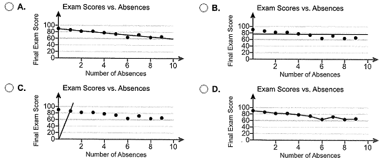
(e) Would it be reasonable to use the least-squares regression line to predict the final exam score for a student who has missed 15 class periods? Why or why not?
A. Yes, because the purpose of finding the regression line is to make predictions outside the scope of the model.
B. No, because the absolute value of the correlation coefficient is less than the critical value for a sample size of n = 10.
C. Yes, because the absolute value of the correlation coefficient is greater than the critical value for a sample size of n = 10.
D. No, because 15 absences is outside the scope of the model.
Q10. The given data represent the total compensation for 10 randomly selected CEOs and their company's stock performance in 2009. Analysis of this data reveals a correlation coefficient of r = - 0.1996. What would be the predicted stock return for a company whose CEO made $15 million? What would be the predicted stock return for a company whose CEO made $25 million?
CEO Compensation and Stock Performance
|
Compensation (millions of dollars
|
Stock Return (%)
|
|
26.07
|
5.97
|
|
12.58
|
30.38
|
|
19.57
|
32.04
|
|
12.97
|
79.84
|
|
11.94
|
- 8.71
|
|
11.42
|
2.91
|
|
25.77
|
4.52
|
|
14.47
|
11.25
|
|
17.27
|
4.35
|
|
14.33
|
11.85
|
View a table of critical values for the correlation coefficient in Q3.
What would be the predicted stock return for a company whose CEO made $15 million?
What would be the predicted stock return for a company whose CEO made $25 million?
Q11. Analyze the residual plot below and identify which, if any, of the conditions for an adequate linear model is not met.
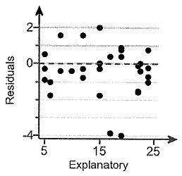
Which of the conditions below might indicate that a linear model would not be appropriate?
- Constant error variance
- None
- Patterned residuals
- Outlier
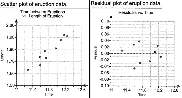
Q12. The following data represent the time between eruptions and the length of eruption for 8 randomly selected geyser eruptions.
|
Time, x
|
Length, y
|
Time, x
|
Length, y
|
|
12.11
|
1.88
|
11.71
|
1.79
|
|
11.59
|
1.67
|
12.26
|
1.91
|
|
11.98
|
1.81
|
11.58
|
1.74
|
|
12.18
|
1.92
|
11.73
|
1.73
|
|
11.28
|
1.63
|
|
|
(1) length of eruption.
time between eruptions.
Complete parts (a) through (c) below.
(a) What type of relation appears to exist between time between eruptions and length of eruption?
A. Linear, negative association
B Linear, positive association
C. A nonlinear pattern.
D. No association.
(b) Does the residual plot confirm that the relation between time between eruptions and length of eruption is linear?
A. Yes. The plot of the residuals shows a discernible pattern, implying that the explanatory and response variables are linearly related.
B. No. The plot of the residuals shows that the spread of the residuals is increasing or decreasing, violating the requirements of a linear model.
C. Yes. The plot of the residuals shows no discernible pattern, so a linear model is appropriate.
D. No. The plot of the residuals shows no discernible pattern, implying that the explanatory and response variables are not linearly related.
(c) The coefficient of determination is found to be 92.5%. Provide an interpretation of this value.
The least squares regression line explains _________ % of the variation in (1) _________ (Type an integer Or a decimal. Do not round.)
Q13. The accompanying data represent the weights of various domestic cars and their gas mileages in the city. The linear correlation coefficient between the weight of a car and its miles per gallon in the city is r = - 0.963. The least-squares regression line treating weight as the explanatory variable and miles per gallon as the response variable is y^ = - 0.0064x + 42.5897.
Data Table
|
Car
|
Weight (pounds), x
|
Miles per Gallon, y
|
Car
|
Weight (pounds), x
|
Miles per Gallon, y
|
|
Car 1
|
3,765
|
19
|
Car 7
|
2,605
|
25
|
|
Car 2
|
3,984
|
18
|
Car 8
|
3,772
|
18
|
|
Car 3
|
3,530
|
20
|
Car 9
|
3,310
|
20
|
|
Car 4
|
3,175
|
22
|
Car 10
|
2,991
|
25
|
|
Car 5
|
2,580
|
26
|
Car 11
|
2,752
|
26
|
|
Car 6
|
3,730
|
18
|
|
|
|
(1) gas mileage
weight
(2) not explained
explained
(3) inappropriate
appropriate
Complete parts (a) through (c) below.
(a) What proportion of the variability in miles per gallon is explained by the relation between weight of the car and miles per gallon?
(b) Construct a residual plot to verify the requirements of the least-squares regression model. Choose the correct graph below.
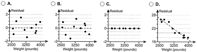
(c) Interpret the coefficient of determination and comment on the adequacy of the linear model.
_______% of the variance in (1) _______is (2) _______ by the linear model. The least-squares regression model appears to be (3) _______, based on the residual plot.
Q14. The data to the right represent the number of chocolate chips per cookie in a random sample of a name brand and a store brand.
|
Name Brand
|
Store Brand
|
|
26
|
29
|
27
|
20
|
16
|
24
|
|
21
|
20
|
20
|
27
|
22
|
22
|
|
33
|
30
|
25
|
30
|
26
|
28
|
|
22
|
23
|
22
|
17
|
27
|
23
|
|
25
|
|
|
33
|
|
|
Complete parts (a) to (c) below.
(a) Draw side-by-side boxplots for each brand of cookie. Label the boxplots "N" for the name brand and "S" for the store brand. Choose the correct answer below.
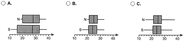
(b) Does there appear to be a difference in the number of chips per cookie?
A. No. There appears to be no difference in the number of chips per cookie.
B. Yes. The name brand appears to have more chips per cookie.
C. Yes. The store brand appears to have more chips per cookie.
D. There is insufficient information to draw a conclusion.
(c) Does one brand have a more consistent number of chips per cookie?
A. Yes. The store brand has a more consistent number of chips per cookie.
B. No. Both brands have roughly the same number of chips per cookie.
C. Yes. The name brand has a more consistent number of chips per cookie.
D. There is insufficient information to draw a conclusion.