Reference no: EM132980640

Question 1. (the Exchange Paradox) You're playing the following monetary game against an opponent, with a referee also taking part; imagine playing this game with two of your friends, which will provide context for the amounts of money that would reasonably be involved in playing it. The referee has two envelopes (numbered 1 and 2 for the sake of this problem, but when the game is played the envelopes have no markings on them), and (without you or your opponent seeing what she does) she (the referee) puts $m in envelope 1 and $2 m in envelope 2 for some m > 0 (let's treat your uncertainty about m as continuous in this problem, even though in practice it would be rounded, let's say to the nearest dollar or penny). You and your opponent each get one of the envelopes at random. You open your envelope secretly and find $x (your opponent also looks secretly in his envelope), and the referee then asks you if you want to trade envelopes with your opponent. You reason that if you trade, you will get either $x/2 or $2x, each with probability 1/2. This makes the expected value of the amount of money you'll get if you trade equal to (1/2) ($x/2) + (1/2) ($2x) = $5x/4, which is greater than the $x you currently have, so you offer to trade. The paradox is that your opponent is capable of making exactly the same calculation. How can the trade be advantageous for both of you? (It can't be.)

The point of this problem is to demonstrate that the above reasoning is flawed from a Bayesian point of view; the conclusion that trading envelopes is always optimal is based on the assumption that there's no information obtained by observing the contents of the envelope you get, and this assumption can be seen to be false when you reason in a Bayesian way. At a moment in time before the game begins, let fM (m) be your (continuous) prior distribution (PDF) for the amount of money M the referee will put in envelope 1, and let X be the amount of money you'll find in your envelope when you open it (when the game is actually played, the observed x, of course, will be data that can be used to decrease your uncertainty about M ).

(a) (preliminary calculations)

(i) Explain why the setup of this problem implies (in a small abuse of formal notation) that P (X = m|M = m) = P (X = 2 m|M = m) = 1 , and use this to show that

P (M = x|X = x) = f_M(x)/fM(x/2)  and P(M = x/2|X = x) = fM(x/2)/fM(x) + fM(x/2)

(ii) Demonstrate from this that the expected value of the amount Y of money in your opponent's envelope, given than you've found $x in the envelope you've opened, is (again in a small abuse of formal notation)

E(Y |X = x) = f_M(x)/(fM(x) + fM(x/2)).(2x)  + fM(x/2)/(fM(x) + fM(x/2))(x/2)

(b) (Bayesian decision theory)

(i) Suppose that for you in this game, money and utility coincide (or at least suppose that utility is linear in money for you with a positive slope). Use Bayesian decision theory, through the principle of maximizing expected utility, to show that you should offer to trade envelopes if and only if

fM(x/2 < 2fM(x)

(ii) If you and two friends (one of whom would serve as the referee) were to actually play this game with real money in the envelopes, it would probably be the case that small amounts of money are more likely to be chosen by the referee than big amounts, which makes it interesting to explore condition (3) for prior distributions that are decreasing (that is, for which fM (m2) < fM (m1) for m2 > m1). Make a sketch of what condition (3) implies for a decreasing fM .

(iii) One possible example of a continuous decreasing family of priors for M is the Exponential distributions indexed by the parameter λ > 0, which represents the reciprocal of the mean of the distribution. Identify the set of conditions in this family of priors, as a function of x and λ, under which it's optimal for you to trade. Does the inequality you obtain in this way make good intuitive sense (in terms of both x and λ)? Explain briefly.

(c) Looking carefully at the correct argument in paragraph 2 of this problem, identify the precise point at which the argument in the first paragraph breaks down, and specify what someone who believes the argument in paragraph 1 is implicitly assuming about the prior distribution fM (m).

Question 2. (practice with joint, marginal and conditional densities) This is a toy problem designed to give you practice in working with a number of the concepts we've examined; in a course like this, every now and then you have to stop looking at real-world problems and just work on technique (it's similar to classical musicians needing to practice scales, in addition to actual pieces of symphonic or chamber music).

Suppose that the continuous random vector X = (X1, X2) has PDF given by

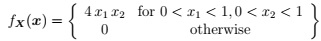
in which x = (x1, x2), and define the random vector Y = (Y1, Y2) with the transformation (Y1 = X1, Y2 = X1 X2).

(a) Are X1 and X2 independent in the joint PDF in equation (4)? Present any relevant calculations to support your answer.

(b) Either work out the correlation ρ(X1, X2) between X1 and X2 or explain why no calculation is necessary in correctly identifying the value of ρ.

(c) (i) Sketch the set SX of possible X values and the image SY of SX under the transformation from X to Y.

(ii) Show that the joint distribution of Y = (Y1, Y2) is

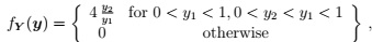
in which y = (y1, y2); verify your calculation by demonstrating that ∫∫_SY f_Y (y) dy = 1.

(d) Work out

(i) the marginal distributions for Y1 and Y2, sketching both distributions and checking that they both integrate to 1;
(ii) the conditional distributions fY1 | Y2 (y1 y2) and fY2 | Y1 (y2 y1), checking that they each integrate to 1; and
(iii) the conditional expectations E(Y1 | Y2) and E(Y2 | Y1); and
(iv) the conditional variances V (Y1 | Y2) and V (Y2 | Y1). (Hint: recall that the variance of a random variable W is just E (W 2) - [E(W )]2.)

(e) Are Y1 and Y2 independent? Present any relevant calculations to support your answer.
(f) Either work out the correlation ρ(Y1, Y2) between Y1 and Y2 or explain why no calculation is necessary in correctly identifying the value of ρ.

Question 3. (moment-generating functions) Distributions may in general be skewed, but there may be conditions on their parameters that make the skewness get smaller or even disappear. This problem uses moment-generating functions (MGFs) to explore that idea for two important discrete distributions, the Binomial and the Poisson.

(a) We saw in class that if X ∼ Binomial(n, p), for 0 < p < 1 and integer n ≥ 1, then the MGF of X is given by

ψ_x (t) = [pe^t + (1 - p)]ⁿ.

for all real t, and we used this to work out the first three moments of X (note that the expression for E (X³) is only correct for n ≥ 3):

E(X) = n p , E(X²) = np[(1 + (n - 1)p],

E(X³)Σ = n p[1 + (n - 2)(n - 1)p² + 3 (n - 1)p],

from which we also found that V (X) = n p(1 - p).

(i) Show that the above facts imply that

skewness(X) = 1 - 2 p/(√n p(1 - p)).

(ii) Under what condition on p, if any, does the skewness vanish? Under what condition on n, if any, does the skewness tend to 0? Explain briefly.

(b) In our brief discussion of stochastic processes we encountered the Poisson distribution: if Y ∼ Poisson(λ), for λ > 0, then the PMF of Y is

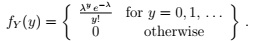
(i) Use this to show that for all real t the MGF of Y is

ψ (t) = e^λ(et-1).

(ii) Use ψY (t) in equation (11) to compute the first three moments of Y, the variance of Y and the skewness of Y. Under what condition on λ, if any, does the skewness either disappear or tend to 0? Explain briefly.

Question 4. (archaeology) Paleontologists estimate the moment in the remote past when a given species became extinct by taking cylindrical, vertical core samples well below the earth's sur- face and looking for the last occurrence of the species in the fossil record, measured in meters above the point P at which the species was known to have first emerged. Letting {yi, i = 1, . . . , n} denote a sample of such distances above P at a random set of locations, the model (Yi|θ) ∼ Uniform(0, θ) (∗) emerges from simple and plausible assumptions. In this model the unknown θ > 0 can be used, through carbon dating, to estimate the species extinction time.

The marginal distribution of a single observation yi in this model may be written

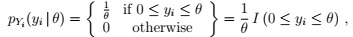
where I(A) = 1 if A is true and 0 otherwise.

(a) Briefly explain why the statement {0 ≤ yi ≤ θ for all i = 1, . . . , n} is equivalent to the statement {m = max (y1, . . . yn) ≤ θ}, and use this to show that the joint distribution of Y = (Y1, . . . , Yn) (given θ) in this model is

fY1,...,Yn (y1, . . . , yn|θ) = I(m ≤ θ)/θn.

(b) Letting the observed values of (Y1, . . . , Yn) be y = (y1, . . . , yn), an important object in both frequentist and Bayesian inferential statistics is the likelihood function A(θ y), which is obtained from the joint distribution of (Y1, . . . , Yn) (given θ) simply by

(1) thinking of fY1,...,Yn (y1, . . . , yn | θ) as a function of θ for fixed y, and
(2) multiplying by an arbitrary positive constant c:

A(θ | y) = c fY (y | θ).

Using this terminology, in part (a) you showed that the likelihood function in this problem is A(θ y) = θ-nI(θ m), where m is the largest of the yi values. Both frequentists and Bayesians are interested in something called the maximum likelihood estimator (MLE) θˆMLE, which is the value of θ that makes A(θ | y) as large as possible.

(i) Make a rough sketch of the likelihood function, and use your sketch to show that the MLE in this problem is θˆMLE = m = max (y1, . . . yn).

(ii) Maximization of a function is often accomplished by setting its first derivative to 0 and solving the resulting equation. Briefly explain why that method won't work in finding the MLE in this case.

(c) A positive quantity W follows the Pareto distri- bution (written W ∼ Pareto(α, β)) if, for parameters α, β > 0, it has PDF

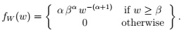
This distribution has mean αβ/α-1 (if α > 1) and variance αβ²/(α-1)²(α-2) (if α > 2).

(i) For frequentists the likelihood function is just a function A(θ y), but for Bayesians it can be regarded as an un-normalized density function for θ. Show that, from this point of view, the likelihood function in this problem corresponds to an un-normalized version of the Pareto(n - 1, m) distribution.

(ii) Bayes's Theorem for a one-dimensional continuous unknown (such as θ in this situation) says that the conditional density fΘ | Y (θ y) for θ given Y = y - which is called the posterior distribution for θ given the data - is a positive (normalizing) constant c times a PDF fΘ(θ) - called the prior distribution for θ - that captures any available information about θ external to the data set, times the likelihood distribution A(θ | y):

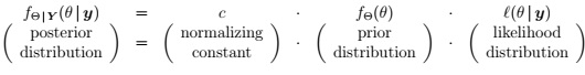
The posterior distribution is the goal of a Bayesian inferential analysis: it summarizes all available information, both external to (prior) and internal to (likelihood) your data set. Show that if the prior distribution for θ in this problem is taken to be (15), under the model ( ) above the posterior distribution is fΘ | Y (θ y) = Pareto [α + n, max(β, m)]. (Bayesian terminology: Note that what just happened was that the product of two Pareto distributions (prior, likelihood) is another Pareto distribution (posterior); a prior distribution that makes this happen is called conjugate to the likelihood in the model.)

(d) In an experiment conducted in the Antarctic in the 1980s to study a particular species of fossil ammonite, the following was a linearly rescaled version of the observed dataset:

y = (y1, . . . , yn) = (2.8, 1.7, 1.0, 5.1, 3.7, 1.5, 4.3, 2.0, 3.2, 2.1, 0.4).

Prior information equivalent to a Pareto distribution specified by the choice (α, β) = (2.5, 4) was available.

(i) Plot the prior, likelihood, and posterior distributions arising from this data set on the same graph, explicitly identifying the three curves.

(ii) Work out the posterior mean and SD (square root of the posterior variance), and use them to complete the following sentence:

On the basis of this prior and data information, the θ value for this species of fossil ammonite is about ____, give or take about _____.

Attachment:- Probability_project.rar