Assignment - Monte Carlo Methods with Financial Applications

Assignment Help Simulation in MATLAB
Reference no: EM132410980

Assignment - Monte Carlo Methods with Financial Applications

The assignment consists of four problems. The objective of the first problem is to test the understanding of some mathematical fundamentals of Monte Carlo simulations. The remaining problems are concerned with option pricing. The options featuring in these problems should be priced in two ways: first, with the help of a direct Monte-Carlo simulation, and then again with Monte Carlo simulation using two different variance reduction techniques (one for each problem). In problem 2 you should use importance sampling but in problems 3 and 4 you may choose yourself which variance reduction techniques to use.

Each solution should include a careful analysis of the results. The quality of both the numerical simulation and the analysis will be decisive in determining the final grade. Both the code, which can be done in computing environment of your choice, and the underlying mathematical reasoning should be clearly presented with detailed comments and arguments.

Tasks - The statements of the problems

1. Let K denote the regular octagon with the vertices

2497_figure.png

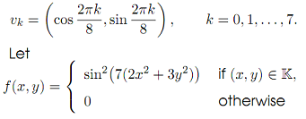
(a) Generate 3000 uniformly distributed points in K and plot the outcome.

(b) Using the acceptance-rejection method generate 3000 points in K which are distributed according to the probability density function of the form f /C, where C > 0 is a normalizing constant, but without calculating the value of C. Plot the outcome.

IMPORTANT: In the option pricing problems below, it is assumed that we are working within the standard risk neutral setting with a constant risk-free rate and the geometric Brownian motion used to model stock prices. For all estimates form approximate confidence intervals (=empirical confidence intervals) at the 95% level of confidence and calculate the approximate relative error (=empirical relative error).

2. Assume that r = 1.9% is the risk-free rate. Consider a range of European call options expiring in 6 months, with different strike prices, all written on the same stock. The price process S(t) of this stock is modeled by a Geometric Brownian Motion with the initial price S(0) = 100 and volatility σ = 25%. Let C(K) denote the price of such an option at time t = 0, expressed as a function of the strike price K > 0. Calculate C(K) for K = 100, 125, 150, 175, 200, 225, 250 using the Black-Scholes formula. Estimate C(K), for the same range of values of K, first using a crude Monte-Carlo approach and then using importance sampling. Explain if there is any advantage of using importance sampling over crude estimates.

3. Let r = 3% be the risk-free rate. Let the prices S1(t) and S2(t) of two stocks evolve according to the geometric Brownian motions with the initial values S1(0) = 75, S2(0) = 50 and the volatilities σ1 = 30% and σ2 = 20%, respectively. Consider the Asian call option with strike price K = 65 expiring in 8 months, written over a simple portfolio of the two stocks given by the formula S(t) = 0.55 S1(t) + 0.45 S2(t). Let ρ denote the correlation coefficient between the Brownian motions W1(t), W2(t) driving S1(t) and S2(t) respectively. First, estimate the price of this option assuming that ρ = 0. Then investigate how changing the value of % to ±0.3, ±0.6, ±0.9 changes the price of this option. You may assume that there are 80 uniformly spaced monitoring dates and that the arithmetic averages are used.

4. Suppose that the risk-free interest rate is r = 2.5%. Consider a stock with the price process S(t) modeled by a geometric Brownian motion with volatility σ = 30%. The stock is assumed to be worth S(0) = 300 at present. Suppose that C(t) denotes the price at time t of the European call option written on this stock expiring in half a year, with strike price L = 300. Estimate the price of the compound put-on-call option with strike price K = 19 and maturing in 3 months, written over that call option. By considering several different values of L below and above 300, investigate how L influences the price of the compound option.

Attachment:- Assignment File.rar

Reference no: EM132410980

Questions Cloud

What does your audience need to know about your problem : Why does your problem need solving? What does your audience need to know about your problem in order to understand and agree with your position?
Protect the value of the bond against rising interest rates : Should the investor buy or sell the forward contract to protect the value of the bond against rising interest rates during the holding period?
Calculate the price of the bond : If the yield to maturity on the bond is 10%, calculate the price of the bond assuming that the bond makes semi-annual coupon interest payments.
Principal and income in tfsa : Savings in TFSA provide no income tax deduction, but the principal and income in TFSA are never taxed, even when withdrawn.
Assignment - Monte Carlo Methods with Financial Applications : Assignment - Monte Carlo Methods with Financial Applications. Generate 3000 uniformly distributed points in K and plot the outcome
How much will be the after tax value of her portfolio : a. How much will be the after tax value of her portfolio after 20years, if she invests in DivOnly? CapG?
What is the complete portfolio expected return : You wish to complete a portfolio with 30 % in T-Bills and the rest in a risky portfolio. The risky portfolio is has 42 % in stocks and the rest in bonds.
Why might different companies have different costs : What are some of the elements that will have an effect on a company's cost of capital? Why might different companies have different costs of capital?
Determine net profit margins : What would you review during the profit and loss budget setting process to determine net profit margins?

Reviews

Write a Review

Simulation in MATLAB Questions & Answers

  Calculate the stress intensity factor

Use the three-parameter zone finite element method or the boundary collocation method to calculate the stress intensity factor K, at the crack tip for the plate

  Build a simulation using newtons laws of motion

Build a new and different simulation of your own using Newtons laws of motion and Show the code and describe how it works

  Write the specification of load mover

Write the specification of LOAD MOVER detailed of the whole design and precise for automatic control section and divide the design into various modules and Is the kernel required if yes which one?

  Design the automatic control section using statecharts

Aim of this project is to design an embedded system which can move loads from one place to another. The system can be operated manually, automatically and wirelessly.

  Need an expert who can model a drill in simulink

Need an expert who can model a drill in Simulink. Working model of a drill needing for an improvment to behave more realistically as a drill to drill through plastic block.

  Project is on load frequency control using fpid

Project is on load frequency control using FPID tuned using GA and PSO algorithm and the system is a two area system.

  Number of packets received with time

Let x be the number of packets received with time -

  Build a matlab based graphical user interface

Build a Matlab based graphical user interface (GUI) that operates in conjunction with a base Matlab/ Simulink simulation program. Any base simulation is considered acceptable.

  Build a matlab based graphical user interface

Build a Matlab based graphical user interface (GUI) that operates in conjunction with a base Matlab/ Simulink simulation program. Any base simulation is considered acceptable.

  Simulate the standardised sum of independent

Simulate the standardised sum of independent and identically distributed variates - Fit a linear regression model as in Q5, and plot your estimates for β0 and β1 as N increases, together with a line indicating their true values. Supply your code.

  Plot the original periodic square wave

Plot the original periodic square wave on the same graph. Comment on the difference between the original periodic square wave and its truncated Fourier series presentation.

  Use matlab to plot the function

Plot the original periodic square wave on the same graph. Comment on the difference between the original periodic square wave and its truncated Fourier series presentation.

Free Assignment Quote

Assured A++ Grade

Get guaranteed satisfaction & time on delivery in every assignment order you paid with us! We ensure premium quality solution document along with free turntin report!

All rights reserved! Copyrights ©2019-2020 ExpertsMind IT Educational Pvt Ltd