Reference no: EM133083918
ENGRD 3200 Engineering Computation - Cornell University
Learning Objective 1: Consider the tradeoff between round-off error and truncation error.
Learning Objective 2: Learn application of numerical differentiation as derived from Taylor Series to both an analytically prescribed function and experimentally measured data.
Learning Objective 3: Develop an understanding of the role of noise in amplifying the error in numerical differentiation.
• The MATLAB codes (please comment your codes).
• The results you get when running your codes for all problems, e.g., plots and numerical values.
Assignment
1. Total Numerical Error
Consider the function f(x)=sin(x) defined over the interval [0,2π].
a) How small do you have to make the distance h between x0 and its neighboring points to compute the first derivative f'(x=x0) at x0=π/4 with an O(h) forward finite difference formula and a relative error of 10-6? Start with a value of h=0.2 and progressively reduce it by a factor of 10 each time until you fall below the desired error threshold. Plot on a log-log diagram the relative error as a function of distance h.
b) In a similar spirit to what we discussed in class, for the above choice of finite difference formula, the truncation error is bounded by Mh/2 where M = max {|f"(ξ)|} and ξ is a point in the neighborhood of x0 (Hint: see Example 4.5 of textbook on how to estimate M). The round-off error is bounded by 2ε/h where ε is the machine epsilon. If you are working with a computer that is limited to single-precision do you expect the same level of accuracy from the numerical differentiation in part (a) of this problem (even with the sufficiently small h you have identified) ? Explain your answer with explicitly repeating the computations of part (a) in single-precision.
2. Numerical Differentiation: Experimental Data with noise
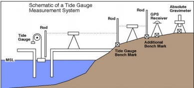
A tidal gauge (see figure below) is a device used by coastal engineers to measure sea-surface elevation over as it varies in time. Differentiation of the sea-surface elevation data may then be used to compute the vertical velocity of the surface and further its associated acceleration. A typical signal recorded over the course of one day is often a near-perfect sinusoid.
Now, let's assume we have a sensor that measures sea surface elevation in meters at a sampling rate of 1 Hz. The local tide has a period of T=12 hours and an amplitude of A=1 m. If our instrument was noise-free it would measure an elevation described by the exact expression f=A cos(2πt/T). Our sensor is very accurate and the manufacturer reports it has a noise level of ±0.1 mm, or 1 part in 10,000). This is a random error so each measurement has a random uncertainty of up to ±0.1 mm.
A file, waveData.mat, with the sampled data is posted on the Canvas website. This file contains a timeseries of the sampled data. You can access the data in Matlab simply by tying: load waveData . The elevation data is in the variable f, and the time (in seconds) is in the variable t. You can type plot(t,f)to see the data. For this problem use this data and numerical differentiation to achieve the following:
a) Plot the 12-hr experimental data timeseries and zoom in to a small section to reveal the random noise.
b) Use an O(h2)-accurate centered finite difference approximation to numerically compute the vertical velocity df/dt of the free surface at every time in your sampled timeseries, with points spaced apart by h=1 sec (neglect the end-points for which you might not be able to form centered differences). Plot your computed result against the exact one (the analytical derivative of f=A cos(2πt/T)). Compute the maximum absolute error within your numerically differentiated dataset.
c) Comment on your result in Part (b). Why does the approximated df/dt look noisier than your measured signal of f ? Are those errors associated with truncation error, round-off error or something else? Does the textbook paradigm of total error = truncation error + round-off error'' completely describe the picture ?
d) In the spirit of minimizing the error, repeat the above exercise using 50 different values of the time step (h) each time. Your goal is to produce a loglog plot like we did in class (see also the attached Matlab demo finiteDifOrder.m) that shows Et (True Error) vs h (step size).
Given that you will plot this using the loglog plot function, space your 50 different h values out logarithmically across the range roughly from 1 second to 1 hour (3600) seconds. To do this easily you can use the logspace function with the range of [1,104] s. For each value of h re- sample the original dataset appropriately (see below). Feel free to round off the non-integer values of the computed logarithmically spaced h values, such that the code built for part (b) may be flexibly used when working with the downsampled signal.
CAREFUL:
• Don't plot your numerically computed timeseries for each value of h. You simply want to hold on to the maximum absolute error for each value of h.
• This part of the problem involves you downsampling your existing dataset. Directions towards this will be given in recitation.
What is the value of h at which your total error is minimized ? For this value of h (roughly 1 hour), generate the same plot as in part (b). Draw the log-log plot of True Eror as a function of
h. Does this plot remind you of a figure in both the textbook and your lecture notes ? What is the dominant component of the error curve to the left of its observed minimum? To the right ?
e) Using an analysis similar to what is done in section 4.4.1 of the textbook (and in your lecture notes), compute a theoretical prediction of the optimal h value that minimizes your total error. How does this value compare to the one empirically obtained from your actual data in part (d)?