Reference no: EM133020981
AE03 Automotive Control and Simulation - Cranfield UniversityAutomotive Control and Simulation
Design Exercise - Cruise Control
Cruise control systems are designed to reduce driver workload on long journeys by maintaining a constant speed. With cruise control, drivers can easily maintain a constant speed without the need to keep the right feet on pedals. (Modern adaptive cruise control also incorporates systems to reduce the speed to avoid collisions, though this is beyond the scope of this exercise - very similar principles would of course be involved!)
In this exercise, you are given a model for the powertrain for a novel electric vehicle and you are asked to design an adaptive cruise control for it. Your input is a ‘wheel torque demand' signal - controlling the total torque applied at the wheels. This can be positive or negative, and the transition between electronic braking and mechanical braking is seamless. You will be asked to explore the model in the exercise, and to explain how it works and what it is representing. The output is a sensor that measures speed in km/h. The sensor - like most real-world sensors - is ‘noisy'.
You will be taken through a design exercise through a series of five questions. You will start by obtaining models suitable for control design, then you will design and test controllers with different techniques. At the end of the assignment, you should have a good practical understanding of the concepts required to design a basic feedback controller. If you look at the intended learning outcomes for this module, you will see that they are covered in full by this assignment. As well as being a ‘summative' assessment, I hope it will be a useful deep learning opportunity.
Question 1. A sensor system for measuring electric current has the following schematic:
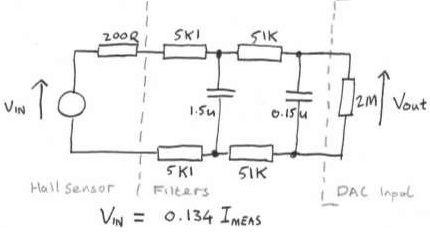
a) Write down the differential equations describing the relationship between the measured current and the output voltage.
b) Without using Simscape (i.e. using integrators and the equation methods taught in lectures) integrating this, implement a Simulink model of the sensor system. By considering a step input of up to 10 A, illustrate the outputs of your model. (Select a suitable timescale for plotting, so that the dynamics are obvious.)
c) Using Laplace transforms, convert your differential equation into a transfer function. Comment on the locations of any poles and zeros and explain how these relate to your observed simulation behaviour.
Question 2. You have been given a set of Simulink models representing the EV powertrain. The main one is called ‘m01_plant_model.slx'.
a) Examine the model, and briefly answer the following questions:
(i) Which (if any) blocks in the model represent nonlinearities? Is the overall model linear or nonlinear?
(ii) How are noise and disturbances modelled?
(iii) What are the model's states?
b) Write a MATLAB program to trim and linearize the version of the model in the file ‘linearization_model.slx' for a steady-state speed of 96 km/h. (You can use the supplied template to help you get started.) Include a listing for your program in your write-up, as well as the transfer function. Use Simulink to compare the linear model with the original nonlinear one.
If you can't solve this question, there is a MATLAB file containing the outputs you would have got, which you can use for the rest of the assignment.
Question 3. Use frequency domain loop-shaping to design a feedback controller for cruise control. Aim for: A stable system, with phase margin of at least 60 degrees.
Steady-state disturbance rejection such that the variation in speed is imperceptible in the Simulink model.
Peak-peak noise in throttle signal that is imperceptible when viewed in the Simulink model. No overshoot in response to a change in set point.
The fastest possible response to a change in set point that (a) doesn't cause an overshoot, and (b) doesn't exceed 0.3 g.
As a control engineer, not every specification you are given will be feasible. If you cannot meet the aims, you should make sensible compromises and describe any trade-offs you have considered.
Your answer should include plots, code samples, etc., that illustrate your design process. You should ensure that you include a Bode plot showing your gain and phase margins, Bode magnitude plots showing T(s), S(s) and C(s) S(s) - if you use a prefilter, you should also include R(s) = T(s) Q(s).
You should test your controller in Simulink, showing a screenshot of your model's top level and relevant plots. Consider small speed changes (a few km/h) and larger demands. How big can the angle be before you see significant effects from nonlinearities in your system?
Question 4. Repeat Question 3, but this time use a PID controller using the following controller structure:
C(s) = kpe(t) + ki∫e(τ)dt + kd de(t)/dt
Design your controller in the frequency domain using proportional, PI and PD weights, as shown in lectures. Do not use a prefilter.
In addition to answering the specifics asked for in Question 3, comment on and the advantages and disadvantages of the simplified PID method compared to the ‘full' frequency-domain loop- shaping method.
(Do not use the MathWorks PID Tuner - it deals with stability margins and time-domain response, but it doesn't make it easy to factor in noise rejection, and the resulting controllers are not ‘pure' PID controllers.)
Question 5. Using the pole placement method, design an observer that can estimate the state variables. Implement this in Simulink and determine how effective it is.
Your answer should include the following:
a) The state space model you use, with the states clearly identified.
b) Relevant code snippets showing how you found the observer gains.
c) Your Simulink model with the observer added. (Don't forget to account for the operating point input u0 in your implementation.)
d) A comparison between your observer's state estimates and the state measurements from the model's measurement bus. Comment on how effective this is.
Attachment:- Automotive Control and Simulation.zip