Example of Transformation of the independent variable:

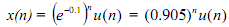
Example: Provided that x(t) = e^-5t u(t) is sampled at 50 Hz, Search an expression for x(n). Plot x(t), x(n) and x(2n). Sketch the spectrum of x(n).

Solution: The sampling time is T = 0.02 sec. Reproducing t with nT we get x(nT) = e^-5nt u(nT ) , or 

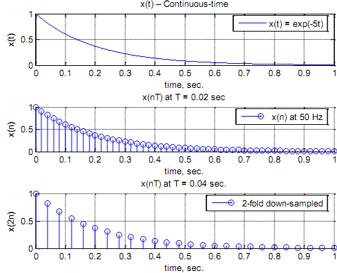
We illustrate below three plots: (1) The continuous-time signal x(t), (2) The sampled (at 50 Hz) version x(n), and (3) x(2n), the 2-fold down-sampled version of x(n); that is similar to sampling x(t) at 25 Hz.

t = 0 : 1/512: 1; xt = exp (-5*t); %x(t) evaluated at 512 points

subplot(3, 1, 1), plot(t, xt); legend ('x(t) = exp(-5t)');

xlabel ('time, sec.'), ylabel('x(t)'); grid; title ('x(t) - Continuous-time')

%

t1 = 0 : 0.02: 1; xn = exp (-5*t1); %Sampled at 50 Hz.

subplot(3, 1, 2), stem(t1, xn); legend ('x(n) at 50 Hz');

xlabel ('time, sec.'), ylabel('x(n)'); grid; title ('x(nT) at T = 0.02 sec')

%

t2 = 0 : 0.04: 1; xt2 = exp (-5*t2); %Sampled at 25 Hz

subplot(3, 1, 3), stem(t2, xt2); legend ('2-fold down-sampled');

xlabel ('time, sec.'), ylabel('x(2n)'); grid; title ('x(nT) at T = 0.04 sec.')

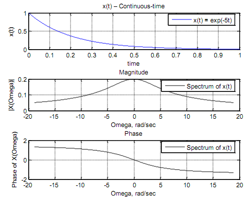
Note that X(s) = L (e^-5t u(t)) = 1 (s + 5) . Defines below is the MATLAB plot of the magnitude spectrum |X(jΩ)| of the continuous-time signal x(t) taking the function plot. Omega is a vector, consequently we need "./" instead of "/" etc. The main point to be prepared here is that X(jΩ) expands asymptotically to ∞, so, strictly speaking, x(t) is not band-limited. Consequently, the spectrum X(ω) of the sampled signal x(n) has some inbuilt aliasing.

t = 0 : 1/512: 1; xt = exp (-5*t); %x(t) evaluated at 512 points

subplot(3, 1, 1), plot(t, xt); legend ('x(t) = exp(-5t)');

xlabel ('time'), ylabel('x(t)'); grid; title ('x(t) - Continuous-time')

%

Omega = -6*pi: pi/256: 6*pi; X = 1./(5.+ j .*Omega);

subplot(3, 1, 2), plot(Omega, abs(X), 'k'); legend ('Spectrum of x(t)');

xlabel ('Omega, rad/sec'), ylabel('|X(Omega)|'); grid; title ('Magnitude')%

subplot(3, 1, 3), plot(Omega, angle(X), 'k'); legend ('Spectrum of x(t)');

xlabel ('Omega, rad/sec'), ylabel('Phase of X(Omega)'); grid; title ('Phase')

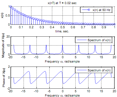
Coming to the discrete-time signal, the spectrum of x(n) = aⁿ u(n) = (0.905)ⁿ u(n) is its DTFT

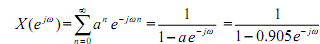
The MATLAB segment is

t1 = 0 : 0.02: 1; xn = exp (-5*t1); %Sampled at 50 Hz.

subplot(3, 1, 1), stem(t1, xn); legend ('x(n) at 50 Hz');

xlabel ('time, sec.'), ylabel('x(n)'); grid; title ('x(nT) at T = 0.02 sec')

%

b = [1]; %Numerator coefficient

a = [1, -0.905]; %Denominator coefficients

w = -6*pi: pi/256: 6*pi; [Xw] = freqz(b, a, w);

subplot(3, 1, 2), plot(w, abs(Xw)); legend ('Spectrum of x(n)');

xlabel('Frequency \omega, rad/sample'), ylabel('Magnitude of X(\omega)'); grid

subplot(3, 1, 3), plot(w, angle(Xw)); legend ('Spectrum of x(n)');

xlabel('Frequency \omega, rad/sample'), ylabel('Phase of X(\omega)'); grid

Email based Example of Transformation of the independent variable assignment help - Example of Transformation of the independent variable homework help at Expertsmind

Are you finding answers for Example of Transformation of the independent variable based questions? Ask Example of Transformation of the independent variable questions and get answers from qualified and experienced  Digital signal processing tutors anytime from anywhere 24x7. We at www.expertsmind.com offer Example of Transformation of the independent variable assignment help -Example of Transformation of the independent variable homework help and  Digital signal processing  problem's solution with step by step procedure.

Why Expertsmind for Digital signal processing assignment help service

1.     higher degree holder and experienced tutors

2.     Punctuality and responsibility of work

3.     Quality solution with 100% plagiarism free answers

4.     On Time Delivery

5.     Privacy of information and details

6.     Excellence in solving Digital signal processing queries in excels and word format.

7.     Best tutoring assistance 24x7 hours