Characteristics of FIR digital filters
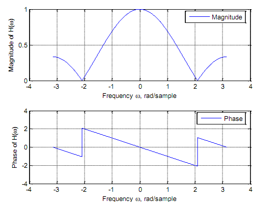
The equations of the three-term moving average filter are shown below

This is a crude low pass filter with simple linear phase, ∠H (ω) = -ω.
%Magnitude and phase response of 3-coefficient moving average filter
%Filter coefficients: h(n) = {1/3, 1/3, 1/3}
b3=[1/3, 1/3, 1/3], a=[1]
w=-pi: pi/256: pi; Hw3=freqz(b3, a, w);
subplot(2, 1, 1), plot(w, abs(Hw3)); legend ('Magnitude');
xlabel('Frequency \omega, rad/sample'), ylabel('Magnitude of H(\omega)'); grid
subplot(2, 1, 2), plot(w, angle(Hw3)); legend ('Phase');
 xlabel('Frequency \omega, rad/sample'), ylabel('Phase of H(\omega)'); grid
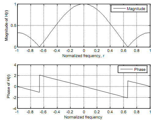
Normalized frequency We describe the r = ω/π. As ω goes from -p to p the value of r goes from-1 to 1. That relates to a frequency range of -Fs/2 to Fs/2 Hz. In terms of the normalized frequency the frequency response of the three-term going average filter goes

%Magnitude and phase response of 3-coefficient moving average filter
%Filter coefficients: h(n) = {1/3, 1/3, 1/3}
subplot(2,1,1); fplot('abs((1/3)*(1+exp(-j*pi*r)+exp(-j*2*pi*r)))', [-1, 1], 'k');
legend ('Magnitude');
xlabel('Normalized frequency, r'); ylabel('Magnitude of H(r)'); grid subplot(2,1,2);fplot('angle((1/3)*(1+exp(-j*pi*r)+exp(- *2*pi*r)))', [-1, 1], 'k'); legend ('Phase');
xlabel('Normalized frequency');ylabel('Phase of H(r)'); grid
We explain below the characteristics of various kinds of FIR filter. The filter length N can be an odd (preferred) or an even number. Further, we are simply interested in linear part of phase. That needs the impulse response to have either odd or even symmetry about its center.
Example: Find the frequency response of the given FIR filters
A. h(n) = {0.25, 0.5, 0.25} Even symmetry
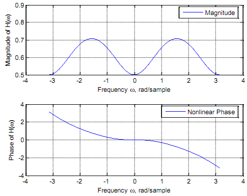
B. h(n) = {0.5, 0.3, 0.2} No symmetry
C. h(n) = {0.25, 0.5, -0.25} No symmetry
D. h(n) = {0.25, 0, -0.25} Odd symmetry
Solution
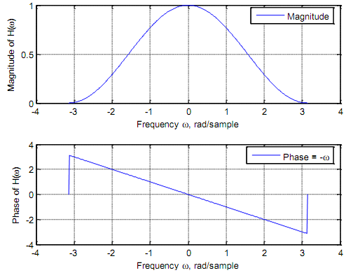
(A) The sequence h(n) = {0.25, 0.5, 0.25} has even symmetry.
%Magnitude and phase response of h(n) = {0.25, 0.5, 0.25}
%Filter coefficients - Even symmetry b3=[0.25, 0.5, 0.25],
a=[1]
w=-pi: pi/256: pi; Hw3=freqz(b3, a, w);
subplot(2, 1, 1), plot(w, abs(Hw3)); legend ('Magnitude');
 xlabel('Frequency \omega, rad/sample'), ylabel('Magnitude of H(\omega)'); grid subplot(2, 1, 2), plot(w, angle(Hw3)); legend ('Phase = -\omega'); xlabel('Frequency \omega, rad/sample'), ylabel('Phase of H(\omega)'); grid
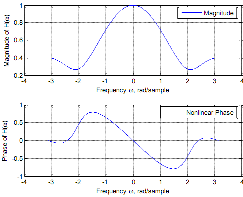
(B) The sequence h(n) = {0.5, 0.3, 0.2}is not symmetric.
%Magnitude and phase response of h(n) = {0.5, 0.3, 0.2}
%Filter coefficients - No symmetry b3=[0.5, 0.3, 0.2],
a=[1]
w=-pi: pi/256: pi; Hw3=freqz(b3, a, w);
 subplot(2, 1, 1), plot(w, abs(Hw3)); legend ('Magnitude');
xlabel('Frequency \omega, rad/sample'), ylabel('Magnitude of H(\omega)'); grid subplot(2, 1, 2), plot(w, angle(Hw3)); legend ('Nonlinear Phase'); xlabel('Frequency \omega, rad/sample'), ylabel('Phase of H(\omega)'); grid
(C) The sequence h(n) = {0.25, 0.5, -0.25} is not symmetric.
%Magnitude and phase response of h(n) = {0.25, 0.5, -0.25}
%Filter coefficients - This is not odd symmetry b3=[0.25, 0.5, -0.25],
a=[1]
w=-pi: pi/256: pi; Hw3=freqz(b3, a, w);
 subplot(2, 1, 1), plot(w, abs(Hw3)); legend ('Magnitude');
xlabel('Frequency \omega, rad/sample'), ylabel('Magnitude of H(\omega)'); grid subplot(2, 1, 2), plot(w, angle(Hw3)); legend ('Nonlinear Phase'); xlabel('Frequency \omega, rad/sample'), ylabel('Phase of H(\omega)'); grid
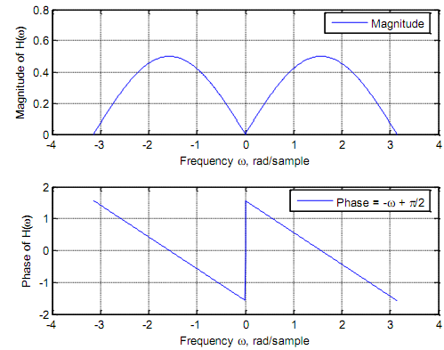
(D) The sequence h(n) = {0.25, 0, -0.25} has odd symmetry.
%Magnitude and phase response of h(n) = {0.25, 0, -0.25}
%Filter coefficients - This is odd symmetry b3=[0.25, 0, -0.25],
a=[1]
w=-pi: pi/256: pi; Hw3=freqz(b3, a, w);
subplot(2, 1, 1), plot(w, abs(Hw3)); legend ('Magnitude');
xlabel('Frequency \omega, rad/sample'), ylabel('Magnitude of H(\omega)'); grid subplot(2, 1, 2), plot(w, angle(Hw3)); legend ('Phase = -\omega + \pi/2 '); xlabel('Frequency \omega, rad/sample'), ylabel('Phase of H(\omega)'); grid
Email based Characteristics of FIR digital filters assignment help - Characteristics of FIR digital filters homework help at Expertsmind
Are you finding answers for Characteristics of FIR digital filters based questions? Ask Characteristics of FIR digital filters questions and get answers from qualified and experienced Digital signal processing tutors anytime from anywhere 24x7. We at www.expertsmind.com offer Characteristics of FIR digital filters assignment help -Characteristics of FIR digital filters homework help and Digital signal processing problem's solution with step by step procedure.
Why Expertsmind for Digital signal processing assignment help service
1. higher degree holder and experienced tutors
2. Punctuality and responsibility of work
3. Quality solution with 100% plagiarism free answers
4. On Time Delivery
5. Privacy of information and details
6. Excellence in solving Digital signal processing queries in excels and word format.
7. Best tutoring assistance 24x7 hours